6 Poison Example: 1 & 2-way ANOVA
Required Packages
library(tidyverse)    # Loads several very helpful 'tidy' packages
library(furniture)    # Nice tables (by our own Tyson Barrett)
library(psych)        # Descriptive helpers
library(pastecs)      # Normality Tests
library(afex)         # Analysis of Factorial Experiments
library(emmeans)      # Estimated marginal means (Least-squares means)
library(ggpubr)
  |
  |                                                                      |   0%
  |
  |........                                                              |  11%
  ordinary text without R code


  |
  |................                                                      |  22%
label: unnamed-chunk-172

  |
  |.......................                                               |  33%
  ordinary text without R code


  |
  |...............................                                       |  44%
label: unnamed-chunk-173

  |
  |.......................................                               |  56%
  ordinary text without R code


  |
  |...............................................                       |  67%
label: unnamed-chunk-174

  |
  |......................................................                |  78%
  ordinary text without R code


  |
  |..............................................................        |  89%
label: unnamed-chunk-175

  |
  |......................................................................| 100%
  ordinary text without R code
[1] "C:\\Users\\A00315~1\\AppData\\Local\\Temp\\RtmpyU9d73\\file35a8572d40e7"6.1 Prepare for Modeling
6.1.1 Ensure the Data is in “long” Format
https://www.guru99.com/r-anova-tutorial.html
The “poison” dataset contains 48 rows and 4 variables:
- ID: Guinea pig identification number
- Time: Survival time of the animal
- poison: Type of poison used: factor level: 1,2 and 3
- treat: Type of treatment used: factor level: 1,2 and 3
Before you start to compute the ANOVA test, you need to prepare the data as follow:
- Import the data from online
- Rename the
idvariable - Declare factors label categories of poison type & treatment
PATH <- "https://raw.githubusercontent.com/guru99-edu/R-Programming/master/poisons.csv"

df_survival <- read.csv(PATH) %>%
  dplyr::rename(id = X) %>%
  dplyr::mutate(poison = factor(poison)) %>%
dplyr::mutate(treat = factor(treat))tibble::glimpse(df_survival)Rows: 48
Columns: 4
$ id <int> 1, 2, 3, 4, 5, 6, 7, 8, 9, 10, 11, 12, 13, 14, 15, 16, 17, 18, …
$ time <dbl> 0.31, 0.45, 0.46, 0.43, 0.36, 0.29, 0.40, 0.23, 0.22, 0.21, 0.1…
$ poison <fct> 1, 1, 1, 1, 2, 2, 2, 2, 3, 3, 3, 3, 1, 1, 1, 1, 2, 2, 2, 2, 3, …
$ treat <fct> A, A, A, A, A, A, A, A, A, A, A, A, B, B, B, B, B, B, B, B, B, …str(df_survival)'data.frame': 48 obs. of 4 variables:
$ id : int 1 2 3 4 5 6 7 8 9 10 ...
$ time : num 0.31 0.45 0.46 0.43 0.36 0.29 0.4 0.23 0.22 0.21 ...
$ poison: Factor w/ 3 levels "1","2","3": 1 1 1 1 2 2 2 2 3 3 ...
$ treat : Factor w/ 4 levels "A","B","C","D": 1 1 1 1 1 1 1 1 1 1 ...6.2 Example 1) Survival Time by Poison Type
6.2.1 Research Question
We want to know if there is a difference between the mean of the survival time according to the type of poison given to the Guinea pig.
6.2.2 Exploratory Data Analysis
6.2.2.1 Summary Statistics
df_survival %>%
  dplyr::group_by(poison) %>%
  furniture::table1("Survival Time" = time,
                    digits = 2,
                    na.rm = FALSE,
                    total = TRUE,
                    output = "markdown",
caption = "Summary of Survival Time by Type of Poisson Used") | Total | 1 | 2 | 3 | |
|---|---|---|---|---|
| n = 48 | n = 16 | n = 16 | n = 16 | |
| Survival Time | ||||
| 0.48 (0.25) | 0.62 (0.21) | 0.54 (0.29) | 0.28 (0.06) |
6.2.2.2 Plot the Observed Data
df_survival %>%
  ggplot(aes(x = poison,
             y = time)) +
  geom_violin(fill = "gray") +
  geom_boxplot(width = .07,
               fill = "white") +
  geom_jitter(position = position_jitter(0.21)) +
  stat_summary(fun = mean,
               geom = "point",
               shape = 18,
               color = "red",
               size = 5) +
  theme_bw() +
  labs(x = "Type of Poison",
y = "Observed Survival Time") 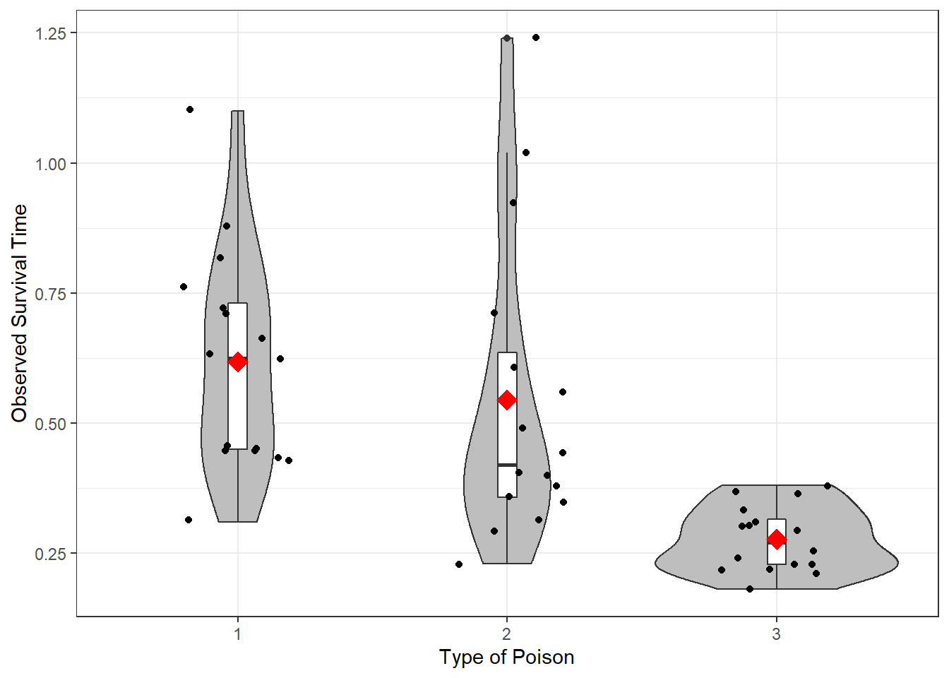
Figure 6.1: Distribution of Survival Time by Poison Type: Violin and Box plots used to Compare Means and Standard Deviations
6.2.2.3 Summary
Things you should notice, but not a firm conclusion yet!
SAMPLE BALANCE (N)
The sample of 48 guinea pigs is balanced between the three poisons. There are the sample number of animals in each group (n = 16).
CENTER (MEANS)
Guinea pigs given Type 3 poison had shorter survival times (M = 0.28), on average, compared to Type 1 (M = 0.48) and Type 2 (M = 0.54).
SPREAD (STANDARD DEVIATIONS)
There was much less variation in survival times among the 16 guinea pics given Type 3 poison (SD = 0.06) compared to the other types (Type 1, SD = 0.21; Type 2, SD = 0.29).
6.2.3 Assumption Checks
6.2.3.1 Independent, Random Samples
The Sample(s) was drawn at random (at least as representative as possible) and the groups are independent of each other.
- Nothing can be done to fix NON-representative samples!
- Can not for with any statistically test
- Lack of independence requires a different model
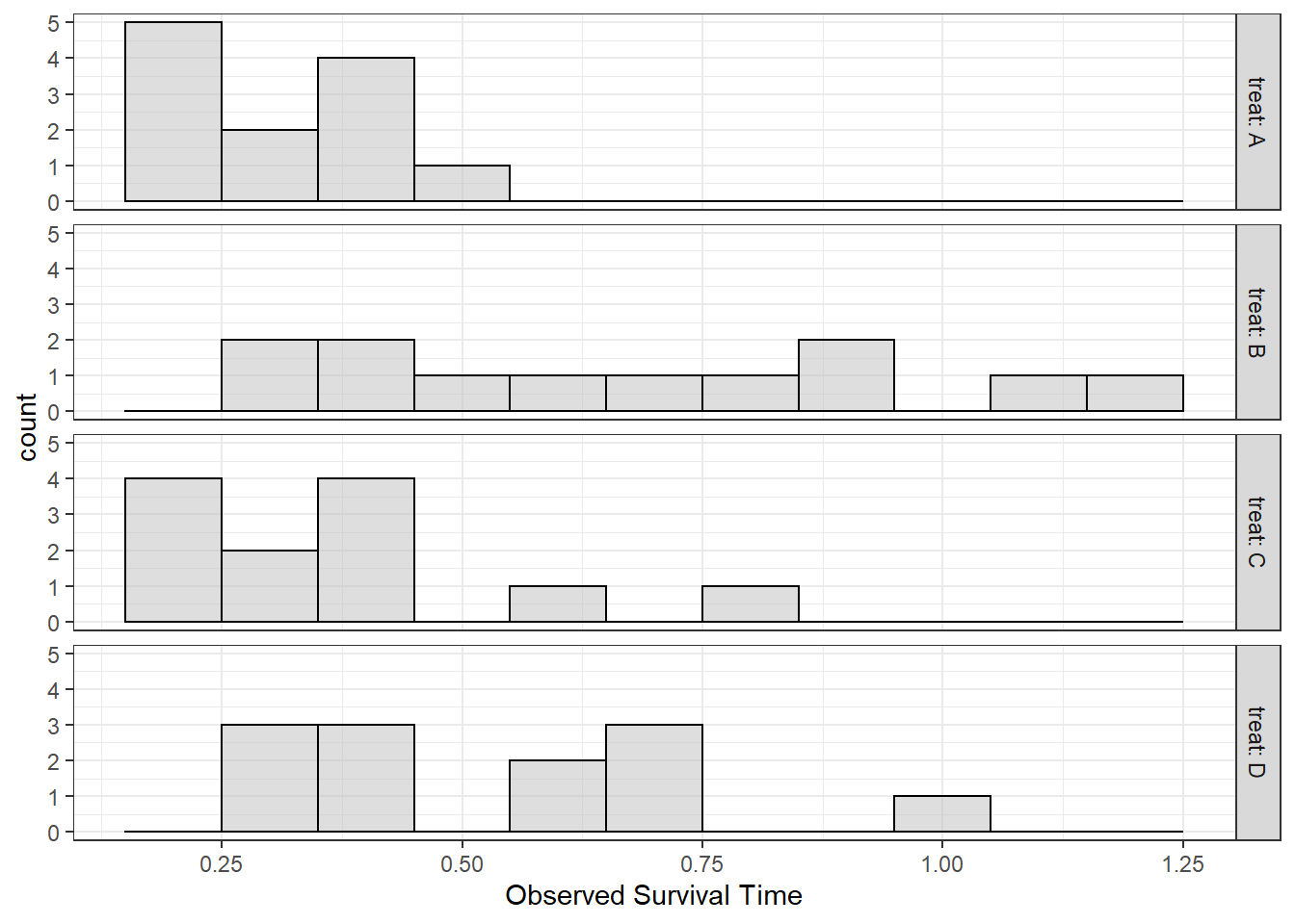
6.2.3.2 Normality of the DV in each Group
df_survival %>%
  ggplot(aes(time)) +
  geom_histogram(binwidth = .05,
                 fill = "gray",
                 color = "black",
                 alpha = .5) +
  facet_grid(poison ~ .,
             labeller = label_both) +
  theme_bw() +
  labs(x = "Observed Survival Time")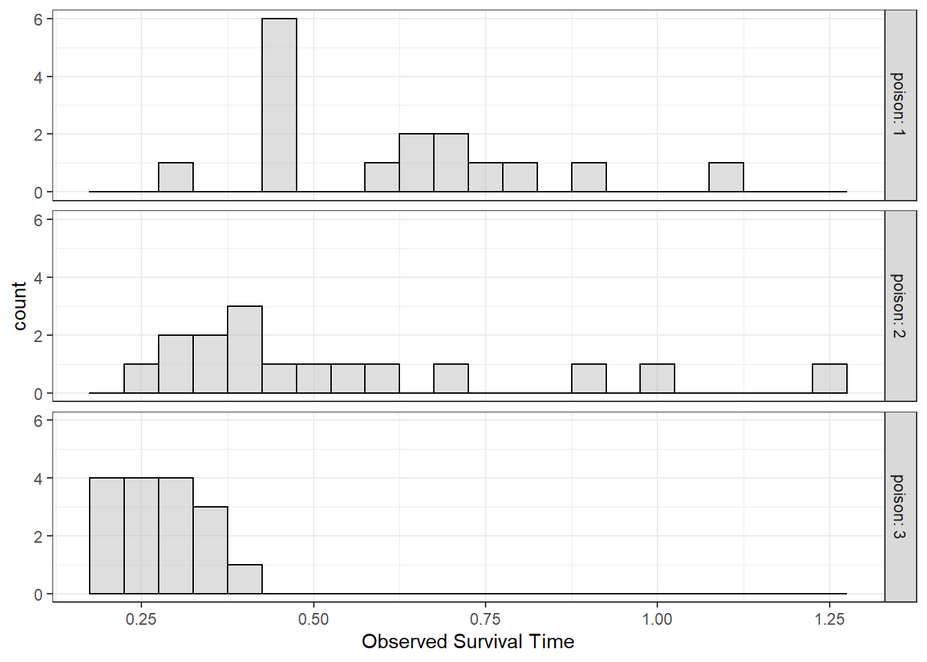
Figure 6.2: Distribution of Survival Time by Poison Type: Histograms used to Judge Normality
df_survival %>%
  ggplot(aes(sample = time)) +
  geom_qq() +
  stat_qq_line() +
  facet_wrap(~ poison,
             labeller = label_both) +
  theme_bw()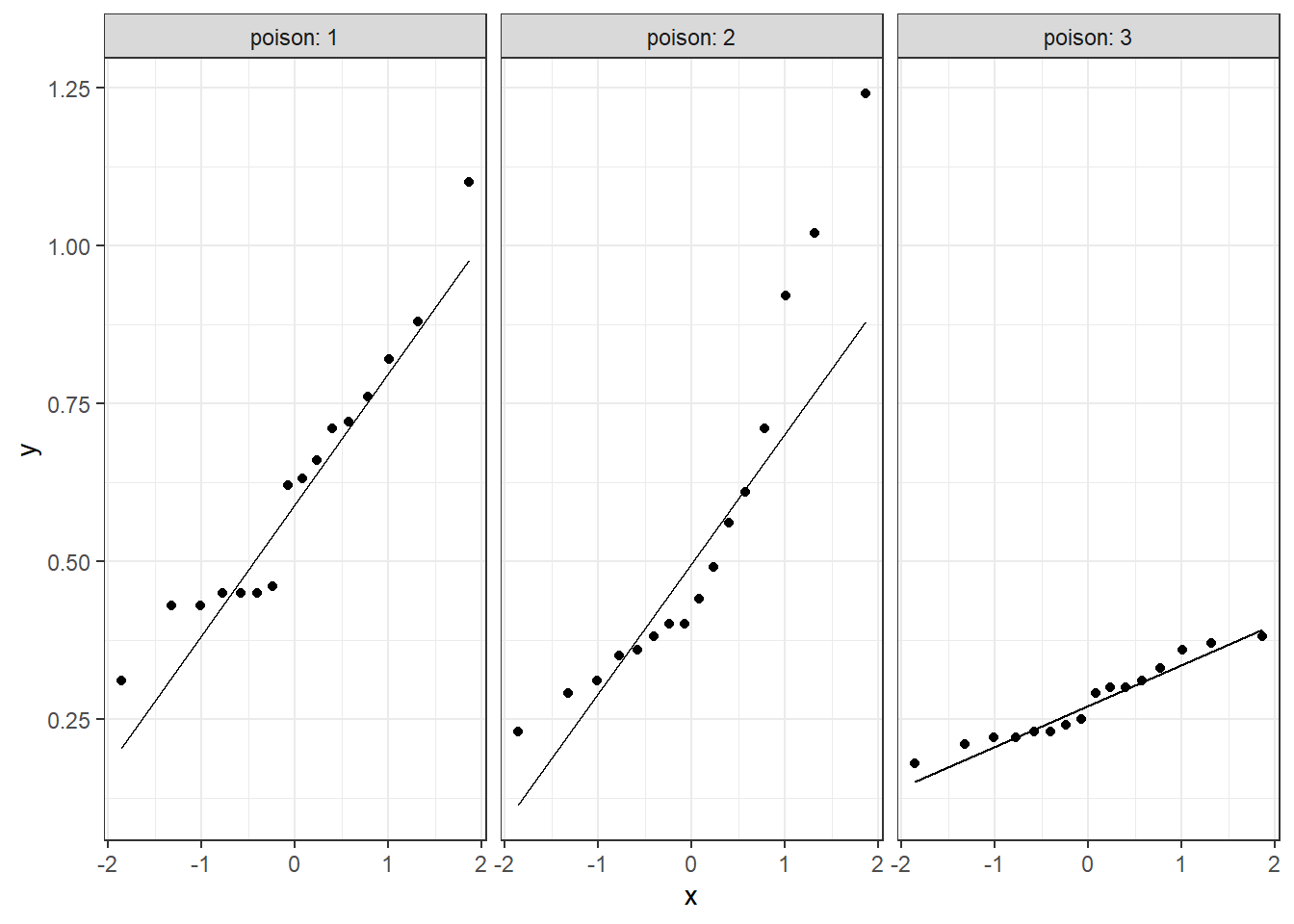
Figure 6.3: Distribution of Survival Time by Poison Type: QQ Plots used to Judge Normality
df_survival %>%
  dplyr::group_by(poison) %>%
  dplyr::summarise(skewness = psych::skew(time),
                   kurtosis = psych::kurtosi(time))
# A tibble: 3 × 3
poison skewness kurtosis
<fct> <dbl> <dbl>
1 1 0.567 -0.543
2 2 1.07 -0.0824
3 3 0.246 -1.38 df_survival %>%
dplyr::group_by(poison) %>%
dplyr::summarise(SW.stat = shapiro.test(time)$statistic,
p.value = shapiro.test(time)$p.value)# A tibble: 3 × 3
poison SW.stat p.value
<fct> <dbl> <dbl>
1 1 0.932 0.266
2 2 0.853 0.0149
3 3 0.936 0.302 df_survival %>%
dplyr::nest_by(poison) %>%
dplyr::summarise(summ = list(pastecs::stat.desc(data$time,
norm = TRUE))) %>%
dplyr::mutate(summ = list(summ %>%
unlist() %>%
data.frame() %>%
dplyr::rename("value" = ".") %>%
tibble::rownames_to_column(var = "stat"))) %>%
tidyr::unnest(summ) %>%
dplyr::filter(stat %in% c("skewness", "skew.2SE",
"kurtosis", "kurt.2SE",
"normtest.W", "normtest.p")) %>%
tidyr::pivot_wider(names_from = stat,
values_from = value)# A tibble: 3 × 7
# Groups: poison [3]
poison skewness skew.2SE kurtosis kurt.2SE normtest.W normtest.p
<fct> <dbl> <dbl> <dbl> <dbl> <dbl> <dbl>
1 1 0.567 0.502 -0.543 -0.249 0.932 0.266
2 2 1.07 0.951 -0.0824 -0.0378 0.853 0.0149
3 3 0.246 0.218 -1.38 -0.634 0.936 0.302 6.2.3.3 Homogeneity of Variance (HOV) in the DV between groups
Since the distribution of survival time might not be normally distributed, Bartlett’s test is not the best.
df_survival %>%
  car::leveneTest(time ~ poison,
                  data = .,
                  center = "mean")
Levene's Test for Homogeneity of Variance (center = "mean")
Df F value Pr(>F)
group 2 8.0941 0.0009937 ***
45
---
Signif. codes: 0 '***' 0.001 '**' 0.01 '*' 0.05 '.' 0.1 ' ' 1df_survival %>%
fligner.test(time ~ poison,
data = .)
    Fligner-Killeen test of homogeneity of variances

data:  time by poison
Fligner-Killeen:med chi-squared = 9.8895, df = 2, p-value = 0.007121
6.2.3.4 Summary
NORMALITY
The distribution of survival time does not seem to be normal based on visual inspection. For poison Type 2, survival time significantly deviates from normality (skew = 1.07, kurtosis = -0.08), W = 0.85, p = .015.
HOMOGENEITY OF VARIANCE
Survival time is significantly less variable for poison Type 3 (SD = 0.06), compared to the others (Type 1, SD = 0.21; Type 2, SD = 0.29), F(2, 45) = 8.09, p < .001.
6.2.4 Fitting One-way ANOVA Model
aov_poison <- df_survival %>%
  afex::aov_4(time ~ poison + (1|id),
              data = .)
6.2.4.1 Basic Output - stored name of model
apa::anova_apa(aov_poison) Effect
1 (Intercept) F(1, 45) = 251.70, p < .001, petasq = .85 ***
2 poison F(2, 45) = 11.79, p < .001, petasq = .34 ***aov_poisonAnova Table (Type 3 tests)
Response: time
Effect df MSE F ges p.value
1 poison 2, 45 0.04 11.79 *** .344 <.001
---
Signif. codes: 0 '***' 0.001 '**' 0.01 '*' 0.05 '+' 0.1 ' ' 16.2.5 Followup-tests
6.2.5.1 Estimated Marginal Means with emmeans::emmeans()
aov_poison %>%
  emmeans::emmeans(~ poison)
poison emmean SE df lower.CL upper.CL
1 0.618 0.0523 45 0.512 0.723
2 0.544 0.0523 45 0.439 0.650
3 0.276 0.0523 45 0.171 0.382
Confidence level used: 0.95 aov_poison %>%
emmeans::emmip(~ poison,
CIs = TRUE) +
theme_bw() +
labs(x = "Type of Poison",
y = "Estmated Marginal Mean: Survival Time")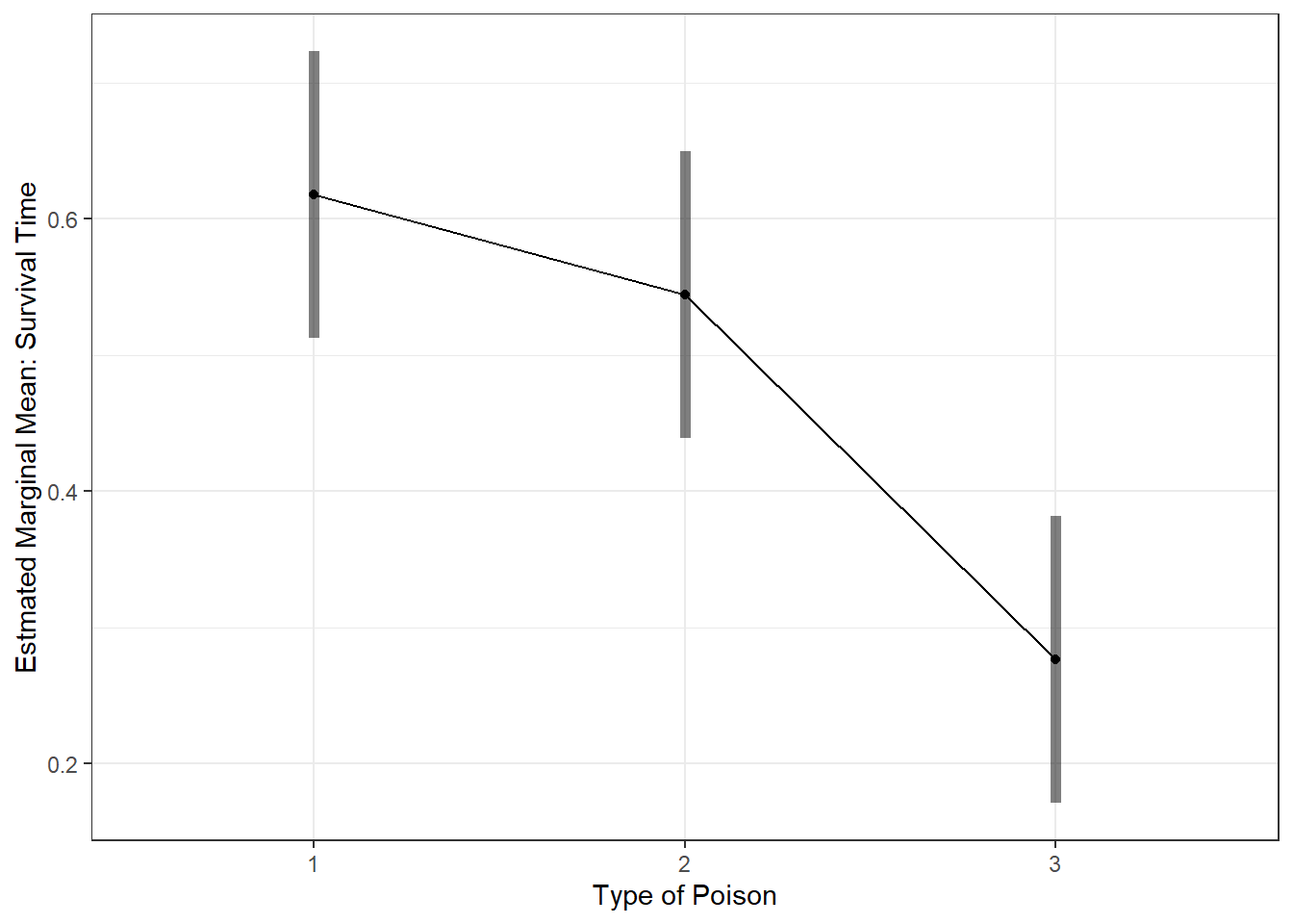
6.2.5.2 All Pairwise Comparisons with pairs()
Pairwise post hoc: Fisher’s LSD adjustment for multiple comparisons
aov_pairs <- aov_poison %>%
  emmeans::emmeans(~ poison) %>%
  pairs(adjust = "none")


aov_pairs
contrast estimate SE df t.ratio p.value
poison1 - poison2 0.0731 0.074 45 0.988 0.3284
poison1 - poison3 0.3412 0.074 45 4.611 <.0001
poison2 - poison3 0.2681 0.074 45 3.623 0.00076.2.5.3 Effect Size for Pairs
aov_eff <- aov_poison %>%
  emmeans::emmeans(~ poison) %>%
  emmeans::eff_size(sigma = sigma(aov_poison$lm),
                    edf = df.residual(aov_poison$lm))

aov_eff
contrast effect.size SE df lower.CL upper.CL
poison1 - poison2 0.349 0.355 45 -0.367 1.07
poison1 - poison3 1.630 0.393 45 0.838 2.42
poison2 - poison3 1.281 0.378 45 0.519 2.04
sigma used for effect sizes: 0.2093
Confidence level used: 0.95 6.2.5.4 Contrast Statements with emmeans::contrast()
Compare the mean of Type 3 to the other two types.
aov_poison %>%
  emmeans::emmeans(~ poison) %>%
  emmeans::contrast(list("1 & 2 vs. 3" = c(1, 1, -2)))
contrast estimate SE df t.ratio p.value
1 & 2 vs. 3 0.609 0.128 45 4.754 <.00016.2.5.5 Summary
PAIRS
Survival time for Type 3 (M = 0.28) is is lower than type 1 (M = 0.62), t(45) = 4.61, p < .001, d = 1.63, and type 2 (M = 0.54), t(45) = 3.62, p < .001, d = 1.28. There is no evidence between types 1 & 2, t(45) = 0.99, p = .328, d = 0.35.
CONTRAST
Survival time for Type 3 (M = 0.28) is is lower than both type 1 (M = 0.62) and type 2 (M = 0.54), t(45) = 4.75, p < .001.
6.2.6 APA Write Up
Note: There are many unkowns regarding the situation of this experiment and can not be include in this write-up.
6.2.6.1 Methods Section
To investigate potency of poisons, 48 guinea pigs were randomized to three types of poison (n = 16) and time till mortality was measured. Survival time (dependent variable) was then subjected to a 1-way independent groups analysis of variance (ANOVA) comparing the three types of poison (independent variable). Prior to analysis, the assumptions of normality and homogeneity of variance were assessed with with Shapiro-Wilks and Levene’s Test respectively. The significant omnibus effect was investigated further with pairwise and appropriate contrast comparisons to determine which of the types different on survival time. Fisher’s method was used for all pairwise tests and effects sizes are given as Cohen’s d-like standardized mean differences.
6.2.6.2 Results Section
The distribution of survival time did not seem to be normal based on visual inspection. For poison Type 2, survival time significantly deviates from normality (skew = 1.07, kurtosis = -0.08), W = 0.85, p = .015. Survival time also was significantly less variable for poison Type 3 (SD = 0.06), compared to the others (Type 1, SD = 0.21; Type 2, SD = 0.29), F(2, 45) = 8.09, p < .001. The ANOVA was still conducted and found statistically significant evidence that survival time do indeed varry by poison type, F(2, 45) = 11.79, p < .001, \(\eta^2\) = 0.34. Specifically, survival time for Type 3 (M = 0.28) was shorter than type 1 (M = 0.62), t(45) = 4.61, p < .001, d = 1.63, and type 2 (M = 0.54), t(45) = 3.62, p < .001, d = 1.28. There was no evidence of a difference in survival time between types 1 & 2, t(45) = 0.99, p = .328, d = 0.35.
Here is a publication worthy plot
aov_poison_label <- dplyr::left_join(data.frame(aov_pairs),
                 data.frame(aov_eff),
                 by = "contrast") %>%
  tidyr::separate(col = contrast,
                  into = c("start", "stop")) %>%
  dplyr::mutate_at(vars(start, stop),
                   stringr::str_sub,
                   start = -1) %>%
  dplyr::mutate(lab = glue::glue("d = {round(effect.size, 2)}, {pval_label_apa(p.value)}"))

aov_poison %>%
  emmeans::emmeans(~ poison) %>%
  data.frame() %>%
  ggplot(aes(x = poison,
             y = emmean)) +
  geom_errorbar(aes(ymin = emmean - SE,
                    ymax = emmean + SE),
                width = .3) +
  geom_point() +
  geom_line(aes(group = 1)) +
  theme_bw() +
  labs(x = "Poison Type",
       y = "Estimated MArginal Mean Survival Time") +
  ggpubr::geom_bracket(data = aov_poison_label %>% dplyr::filter(p.value < .06),
               aes(xmin = start,
                   xmax = stop,
                   label = lab),
               y.position = 0.7,
               step.increase = -0.15,
type = "text") 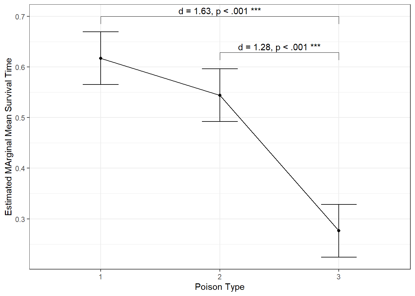
6.3 Example 2) Survival Time by Treatment Type
6.3.1 Parepare for Analysis
Our objective is to test the following assumption:
H_0: There is no difference in survival time average between group
H_a: The survival time average is different for at least one group.
In other words, you want to know if there is a statistical difference between the mean of the survival time according to the type of treatment given to the Guinea pig.
Variables:
idGuinea pig identification numbertreattreatment type, 4-level IV (independent groups)timesurvival time, continuous DV (Y, outcome)
Note: ignore
poisonfor now
6.3.1.1 Compute Summary Statistics
Second, check the summary statistics for each of the \(k=4\) groups.
df_survival %>%
  dplyr::group_by(treat) %>%   # divide into groups
  furniture::table1("Survival Time" = time,
                    digits = 2,      # gives M(SD)
                    na.rm = FALSE,
                    total = TRUE,
                    output = "markdown",
caption = "Summary of Survival Time by Type of Treatment Used") | Total | A | B | C | D | |
|---|---|---|---|---|---|
| n = 48 | n = 12 | n = 12 | n = 12 | n = 12 | |
| Survival Time | |||||
| 0.48 (0.25) | 0.31 (0.10) | 0.68 (0.32) | 0.39 (0.17) | 0.53 (0.22) |
Interpretion:
6.3.1.2 Plot the Raw Data
Plot the data to eyeball the potential effect. Remember the center line in each box represents the median, not the mean. I have added a red diamond on the mean survival time for each type of poison.
df_survival %>%
  ggplot(aes(x = treat,
             y = time)) +
  geom_violin(fill = "gray") +
  geom_boxplot(width = .07,
               fill = "white") +
  geom_jitter(position = position_jitter(0.21)) +
  stat_summary(fun = mean,
               geom = "point",
               shape = 18,
               color = "red",
               size = 5) +
  theme_bw() +
  labs(x = "Type of Treatment",
       y = "Observed Survival Time")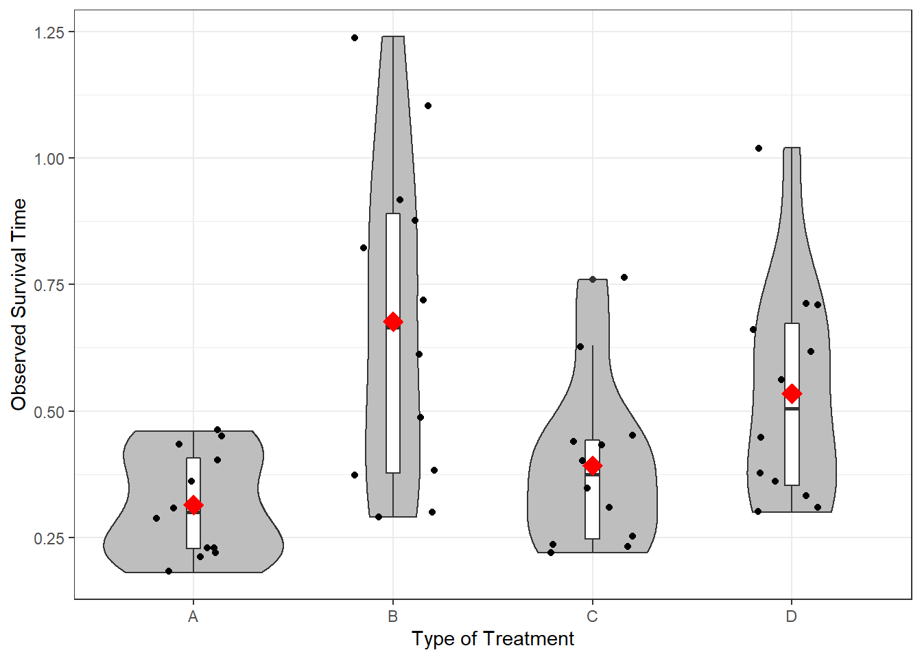
6.3.2 Fitting One-way ANOVA Model
aov_treat <- df_survival %>%
  afex::aov_4(time ~ treat + (1|id),
data = .)6.3.3 Followup-tests
6.3.3.1 Estimated Marginal Means with emmeans::emmeans()
aov_treat %>%
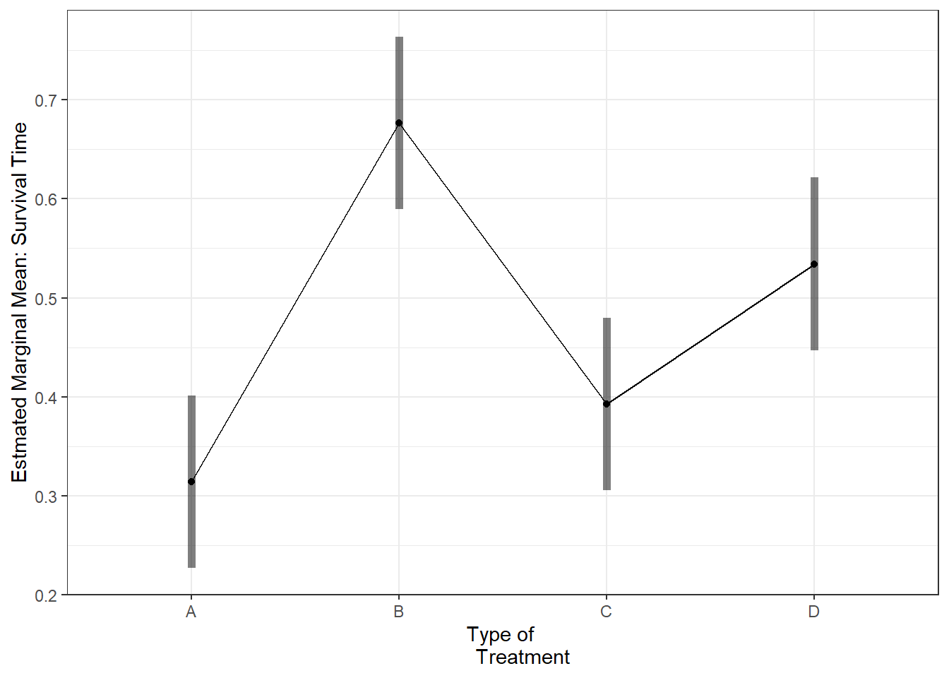
emmeans::emmeans(~ treat) # Calculate Estimated Marginal Means treat emmean SE df lower.CL upper.CL
A 0.314 0.0628 44 0.188 0.441
B 0.677 0.0628 44 0.550 0.803
C 0.393 0.0628 44 0.266 0.519
D 0.534 0.0628 44 0.408 0.661
Confidence level used: 0.95 aov_treat %>%
emmeans::emmip(~ treat,
CIs = TRUE) +
theme_bw() +
labs(x = "Type of Treatment",
y = "Estmated Marginal Mean: Survival Time")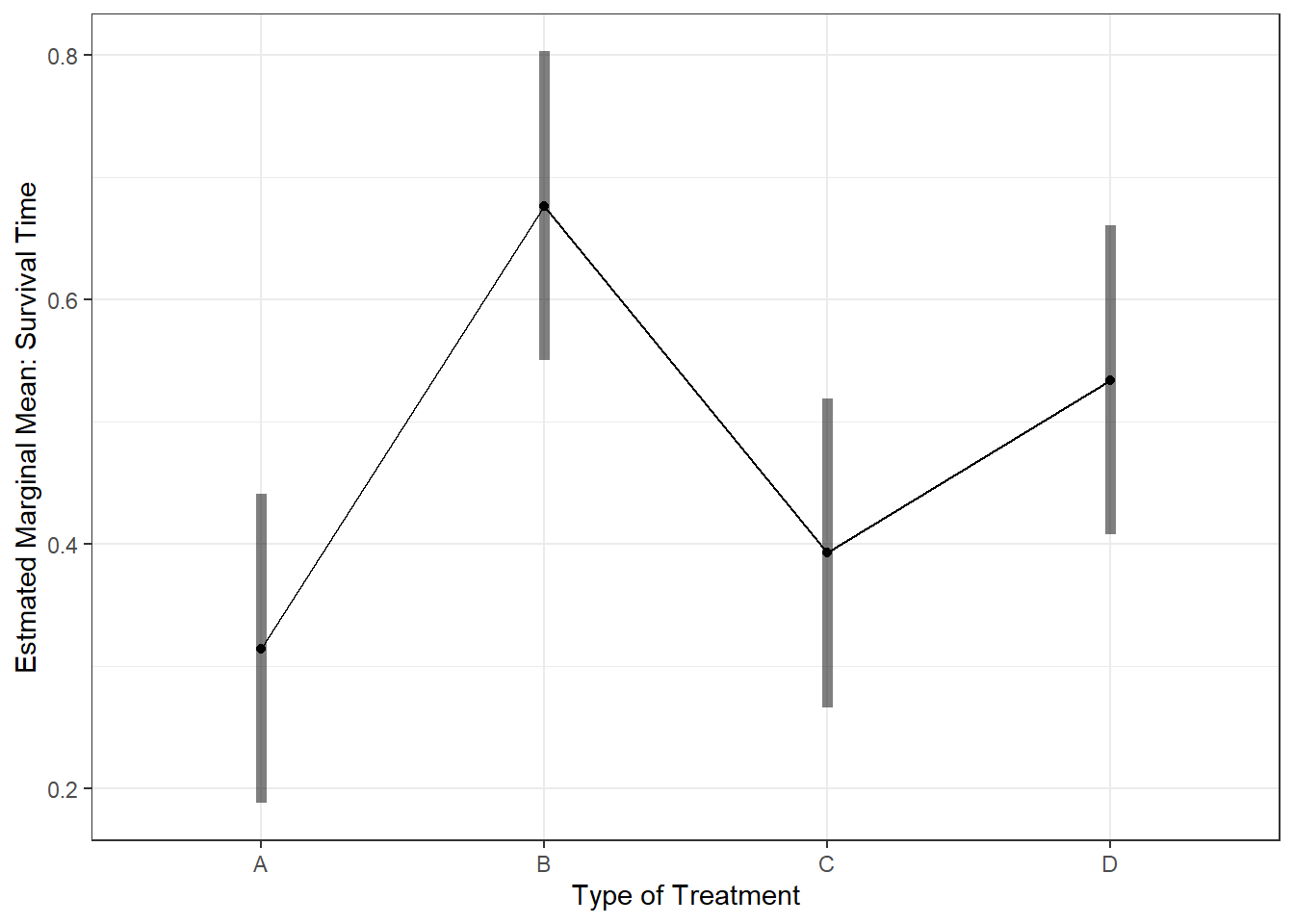
6.3.3.2 All Pairwise Comparisons with pairs()
Pairwise post hoc: Fisher’s LSD adjustment for multiple comparisons
aov_treat %>%
  emmeans::emmeans(~ treat) %>%        # Calculate Estimated Marginal Means
  pairs(adjust = "none")                  # Is each pair signif different?
contrast estimate SE df t.ratio p.value
A - B -0.3625 0.0888 44 -4.080 0.0002
A - C -0.0783 0.0888 44 -0.882 0.3827
A - D -0.2200 0.0888 44 -2.476 0.0172
B - C 0.2842 0.0888 44 3.198 0.0026
B - D 0.1425 0.0888 44 1.604 0.1159
C - D -0.1417 0.0888 44 -1.595 0.11806.4 Example 3) Survival Time by Both Poisson & Treatment Type
6.4.1 Parepare for Analysis
Our objective is to test the following assumption:
H_0: There is no difference in survival time average between group
H_a: The survival time average is different for at least one group
In other words, you want to know if there is a statistical difference between the mean of the survival time according to BOTH type of poisons and treatment given to the Guinea pig.
Variables:
idGuinea pig identification numberpoisonpoison type, 3-level IV (independent groups)treattreatment type, 4-level IV (independent groups)timesurvival time, continuous DV (Y, outcome)
6.4.1.1 Compute Summary Statistics
Second, check the summary statistics for each of the \(k\) groups.
df_survival %>%
  dplyr::group_by(treat, poison) %>%   # divide into groups
  dplyr::summarise(n = n(),
                   mean = mean(time),
                   sd = sd(time)) %>%
gt::gt(caption = "Summary of Survival Time by Type of Treatment Used")| poison | n | mean | sd |
|---|---|---|---|
| A | |||
| 1 | 4 | 0.4125 | 0.06946222 |
| 2 | 4 | 0.3200 | 0.07527727 |
| 3 | 4 | 0.2100 | 0.02160247 |
| B | |||
| 1 | 4 | 0.8800 | 0.16083117 |
| 2 | 4 | 0.8150 | 0.33630343 |
| 3 | 4 | 0.3350 | 0.04654747 |
| C | |||
| 1 | 4 | 0.5675 | 0.15671099 |
| 2 | 4 | 0.3750 | 0.05686241 |
| 3 | 4 | 0.2350 | 0.01290994 |
| D | |||
| 1 | 4 | 0.6100 | 0.11284207 |
| 2 | 4 | 0.6675 | 0.27097048 |
| 3 | 4 | 0.3250 | 0.02645751 |
6.4.1.2 Plot the Raw Data
Third, plot the data to eyeball the potential effect. Remember the center line in each box represents the median, not the mean. I have added a red diamond on the mean survival time for each type of poison.
df_survival %>%
  ggplot(aes(x = treat,
             y = time)) +
  geom_violin(fill = "gray") +
  geom_boxplot(width = .07,
               fill = "white") +
  geom_jitter(position = position_jitter(0.21)) +
  stat_summary(fun = mean,
               geom = "point",
               shape = 18,
               color = "red",
               size = 5) +
  theme_bw() +
  labs(x = "Type of Treatment",
       y = "Observed Survival Time") +
  facet_wrap(~ poison, labeller = label_both)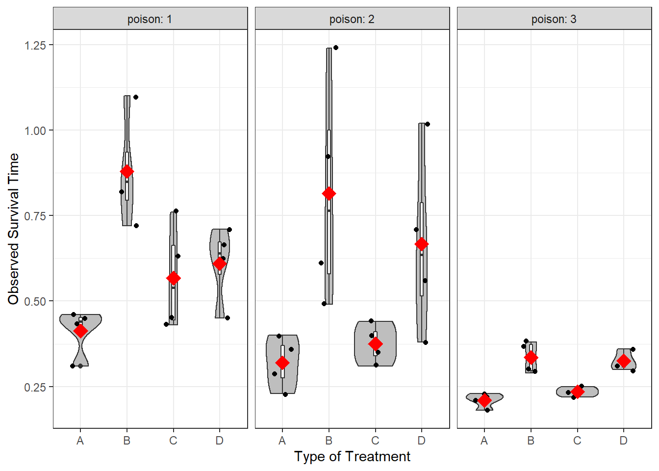
6.4.1.3 Assumption Check: Normality
df_survival %>%
  ggplot(aes(time)) +
  geom_density(fill = "gray",
               alpha = .5) +
  facet_grid(treat ~ poison,
             labeller = label_both) +
  theme_bw() +
  labs(x = "Observed Survival Time")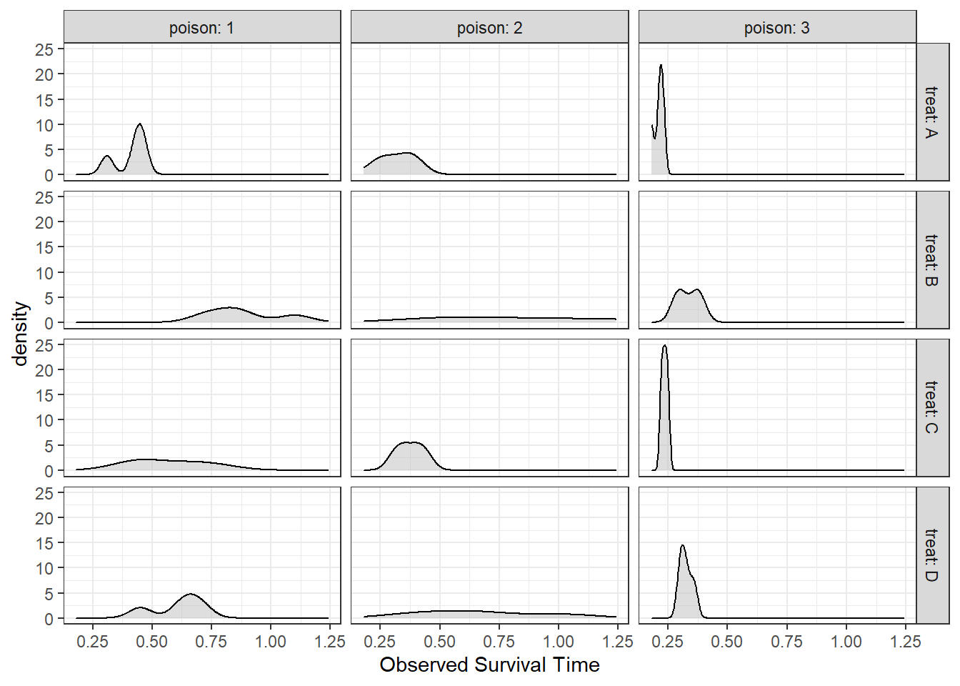
6.4.1.4 Assumption Check: HOV
Levene’s Test of HOV
df_survival %>%
  car::leveneTest(time ~ treat*poison,
                  data = .,
                  center = "mean")
Levene's Test for Homogeneity of Variance (center = "mean")
Df F value Pr(>F)
group 11 4.8535 0.0001442 ***
36
---
Signif. codes: 0 '***' 0.001 '**' 0.01 '*' 0.05 '.' 0.1 ' ' 16.4.2 Fitting Two-way ANOVA Model
aov_survival2 <- df_survival %>%
  afex::aov_4(time ~ poison*treat + (1|id),
              data = .)
6.4.2.1 Basic Output - stored name of model
aov_survival2Anova Table (Type 3 tests)
Response: time
Effect df MSE F ges p.value
1 poison 2, 36 0.02 23.22 *** .563 <.001
2 treat 3, 36 0.02 13.81 *** .535 <.001
3 poison:treat 6, 36 0.02 1.87 .238 .112
---
Signif. codes: 0 '***' 0.001 '**' 0.01 '*' 0.05 '+' 0.1 ' ' 16.4.2.2 Fuller Output - add $Anova on model name
aov_survival2$AnovaAnova Table (Type III tests)
Response: dv
Sum Sq Df F value Pr(>F)
(Intercept) 11.0304 1 495.9194 < 2.2e-16 ***
poison 1.0330 2 23.2217 3.331e-07 ***
treat 0.9212 3 13.8056 3.777e-06 ***
poison:treat 0.2501 6 1.8743 0.1123
Residuals 0.8007 36
---
Signif. codes: 0 '***' 0.001 '**' 0.01 '*' 0.05 '.' 0.1 ' ' 16.4.3 Followup-tests
6.4.3.2 All Pairwise Comparisons for Main Effects of Poison
aov_survival2 %>%
  emmeans::emmeans(~ poison) %>%        # Calculate Estimated Marginal Means
  pairs(adjust = "none")                  # Is each pair signif different?
contrast estimate SE df t.ratio p.value
poison1 - poison2 0.0731 0.0527 36 1.387 0.1740
poison1 - poison3 0.3412 0.0527 36 6.472 <.0001
poison2 - poison3 0.2681 0.0527 36 5.085 <.0001
Results are averaged over the levels of: treat aov_survival2 %>%
emmeans::emmip( ~ poison,
CIs = TRUE) +
theme_bw() +
labs(x = "Type of Poison",
y = "Estmated Marginal Mean: Survival Time")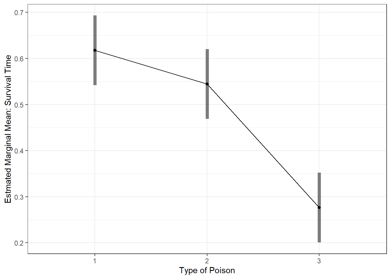
6.4.3.3 All Pairwise Comparisons for Main Effects of Treatment
aov_survival2 %>%
  emmeans::emmeans(~ treat) %>%        # Calculate Estimated Marginal Means
  pairs(adjust = "tukey")                  # Is each pair signif different?
contrast estimate SE df t.ratio p.value
A - B -0.3625 0.0609 36 -5.954 <.0001
A - C -0.0783 0.0609 36 -1.287 0.5772
A - D -0.2200 0.0609 36 -3.613 0.0049
B - C 0.2842 0.0609 36 4.667 0.0002
B - D 0.1425 0.0609 36 2.340 0.1077
C - D -0.1417 0.0609 36 -2.327 0.1108
Results are averaged over the levels of: poison
P value adjustment: tukey method for comparing a family of 4 estimates aov_survival2 %>%
emmeans::emmip( ~ treat,
CIs = TRUE) +
theme_bw() +
labs(x = "Type of
Treatment",
y = "Estmated Marginal Mean: Survival Time")