14 Count Outcome Regression - Ex:
library(tidyverse)
library(haven)        # read in SPSS dataset
library(furniture)    # nice table1() descriptives
library(stargazer)    # display nice tables: summary & regression
library(texreg)       # Convert Regression Output to LaTeX or HTML Tables
library(psych)        # contains some useful functions, like headTail
library(car)          # Companion to Applied Regression
library(sjPlot)       # Quick plots and tables for models
library(glue)         # Interpreted String Literals

library(DescTools)    # Tools for Descriptive Statistics
library(texreghelpr)  # Helper Functions for generalized models

library(pscl)         # Political Science Computational Laboratory (ZIP)
14.1 Background
This dataset comes from John Hoffman’s textbook: Regression Models for Categorical, Count, and Related Variables: An Applied Approach (2004) Amazon link, 2014 edition
14.1.1 Raw Dataset
data_gss <- haven::read_spss("https://raw.githubusercontent.com/CEHS-research/data/master/Hoffmann_datasets/gss.sav") %>%
  haven::as_factor()

data_gss %>%
  dplyr::select(volteer, female, nonwhite, educate, income) %>%
  head()
# A tibble: 6 x 5
volteer female nonwhite educate income
<dbl> <fct> <fct> <dbl> <dbl>
1 0 female non-white 12 10
2 0 male white 17 2
3 0 female non-white 8 NA
4 1 female white 12 NA
5 1 male white 12 12
6 0 female white NA NA14.2 Exploratory Data Analysis
14.2.1 Entire Sample
--------------------------------------
 volteer Freq CumFreq Percent CumPerc
 0       2376 2376    81.85%  81.85%
 1       286  2662    9.85%   91.70%
 2       133  2795    4.58%   96.28%
 3       64   2859    2.20%   98.48%
 4       19   2878    0.65%   99.14%
 5       11   2889    0.38%   99.52%
 6       7    2896    0.24%   99.76%
 7       6    2902    0.21%   99.97%
 9       1    2903    0.03%   100.00%
-------------------------------------- volteer
Min. :0.0000
1st Qu.:0.0000
Median :0.0000
Mean :0.3334
3rd Qu.:0.0000
Max. :9.0000 
14.2.2 By Sex
data_gss %>%
  dplyr::group_by(female) %>%
  furniture::table1(factor(volteer),
                    digits = 4,
                    total = TRUE)
--------------------------------------------------------
                                    female
                 Total        male         female
                 n = 2903     n = 1285     n = 1618
 factor(volteer)
    0            2376 (81.8%) 1057 (82.3%) 1319 (81.5%)
    1            286 (9.9%)   132 (10.3%)  154 (9.5%)
    2            133 (4.6%)   50 (3.9%)    83 (5.1%)
    3            64 (2.2%)    26 (2%)      38 (2.3%)
    4            19 (0.7%)    10 (0.8%)    9 (0.6%)
    5            11 (0.4%)    4 (0.3%)     7 (0.4%)
    6            7 (0.2%)     5 (0.4%)     2 (0.1%)
    7            6 (0.2%)     1 (0.1%)     5 (0.3%)
    9            1 (0%)       0 (0%)       1 (0.1%)
--------------------------------------------------------
data_gss %>%
dplyr::group_by(female) %>%
furniture::table1(volteer,
digits = 4,
total = TRUE,
test = TRUE)
-----------------------------------------------------------------
                                  female
         Total           male            female          P-Value
         n = 2903        n = 1285        n = 1618
 volteer                                                 0.365
         0.3334 (0.8858) 0.3167 (0.8493) 0.3467 (0.9139)
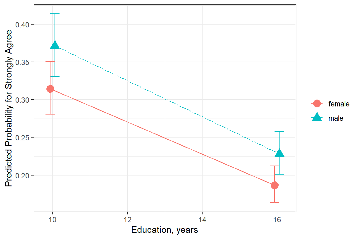
-----------------------------------------------------------------
14.3 Poisson Reression
14.3.1 Single Predictor: Sex
14.3.1.1 Fit the model
glm_possion_1 <- glm(volteer ~ female,
                     data = data_gss,
                     family = poisson(link = "log"))

summary(glm_possion_1)
Call:
glm(formula = volteer ~ female, family = poisson(link = "log"),
    data = data_gss)

Deviance Residuals:
    Min       1Q   Median       3Q      Max
-0.8327  -0.8327  -0.7959  -0.7959   6.4273

Coefficients:
             Estimate Std. Error z value Pr(>|z|)
(Intercept)  -1.14970    0.04957  -23.19   <2e-16 ***
femalefemale  0.09048    0.06511    1.39    0.165
---
Signif. codes:  0 '***' 0.001 '**' 0.01 '*' 0.05 '.' 0.1 ' ' 1

(Dispersion parameter for poisson family taken to be 1)

    Null deviance: 3658.1  on 2902  degrees of freedom
Residual deviance: 3656.2  on 2901  degrees of freedom
AIC: 4924.1

Number of Fisher Scoring iterations: 6
Note: The deviance residuals range as high as 6.47!!!
14.3.1.2 Marginal Estimates
Note: Results are given on the log (not the response) scale
 female emmean     SE  df asymp.LCL asymp.UCL
 male    -1.15 0.0496 Inf     -1.25    -1.053
 female  -1.06 0.0422 Inf     -1.14    -0.976

Results are given on the log (not the response) scale.
Confidence level used: 0.95
Note: These means are on the original scale (number of volunteer activities in the past year). These standard errors are called “delta-method standard errors”
# Hoffmann Example 6.4 (continued...)
ggeffects::ggpredict(model = glm_possion_1,
                     terms = c("female")) %>%
  data.frame()
# A tibble: 2 x 6
x predicted std.error conf.low conf.high group
<fct> <dbl> <dbl> <dbl> <dbl> <fct>
1 male 0.317 0.0496 0.287 0.349 1
2 female 0.347 0.0422 0.319 0.377 1 14.3.1.3 Pairwise Post Hoc Test
 contrast      estimate     SE  df z.ratio p.value
 male - female  -0.0905 0.0651 Inf -1.390  0.1647

Results are given on the log (not the response) scale.
14.3.1.4 Parameter Estimates
Coefficients are in terms of the LOG of the number of times a person volunteers per year.
 (Intercept) femalefemale
 -1.14970081   0.09047562
Exponentiating the coefficients (betas) returns the values to the original scale (number of times a person volunteers per year) and is refered to as the incident rate ratio IRR.
 (Intercept) femalefemale
   0.3167315    1.0946948
# Hoffmann Example 6.4
texreg::knitreg(list(glm_possion_1,
texreghelpr::extract_glm_exp(glm_possion_1,
include.aic = FALSE,
include.bic = FALSE,
include.loglik = FALSE,
include.deviance = FALSE,
include.nobs = FALSE)),
custom.model.names = c("b (SE)", "RR [95% CI]"),
custom.coef.map = list("(Intercept)" ="Intercept",
femalefemale = "Female vs. Male"),
caption = "GLM: Simple Possion Regression",
single.row = TRUE,
digits = 3)| b (SE) | RR [95% CI] | |
|---|---|---|
| Intercept | -1.150 (0.050)*** | 0.317 [0.287; 0.349]* |
| Female vs. Male | 0.090 (0.065) | 1.095 [0.964; 1.244]* |
| AIC | 4924.135 | |
| BIC | 4936.082 | |
| Log Likelihood | -2460.068 | |
| Deviance | 3656.198 | |
| Num. obs. | 2903 | |
| p < 0.001; p < 0.01; p < 0.05 (or Null hypothesis value outside the confidence interval). | ||
14.3.2 Multiple Predictors
14.3.2.1 Fit the model
# Hoffmann Example 6.5
glm_possion_2 <- glm(volteer ~ female + nonwhite + educate + income,
                     data = data_gss,
                     family = poisson(link = "log"))

summary(glm_possion_2)
Call:
glm(formula = volteer ~ female + nonwhite + educate + income,
    family = poisson(link = "log"), data = data_gss)

Deviance Residuals:
    Min       1Q   Median       3Q      Max
-1.3061  -0.8864  -0.7597  -0.6064   5.8489

Coefficients:
                  Estimate Std. Error z value Pr(>|z|)
(Intercept)       -3.15830    0.24479 -12.902  < 2e-16 ***
femalefemale       0.26132    0.07785   3.357 0.000789 ***
nonwhitenon-white -0.28038    0.10838  -2.587 0.009681 **
educate            0.10280    0.01443   7.123 1.05e-12 ***
income             0.05683    0.01566   3.628 0.000286 ***
---
Signif. codes:  0 '***' 0.001 '**' 0.01 '*' 0.05 '.' 0.1 ' ' 1

(Dispersion parameter for poisson family taken to be 1)

    Null deviance: 2566.8  on 1943  degrees of freedom
Residual deviance: 2465.5  on 1939  degrees of freedom
  (959 observations deleted due to missingness)
AIC: 3380.9

Number of Fisher Scoring iterations: 6
14.3.2.2 Parameter Estimates
Coefficients are in terms of the LOG of the number of times a person volunteers per year.
      (Intercept)      femalefemale nonwhitenon-white           educate
      -3.15830174        0.26132182       -0.28037733        0.10280183
           income
       0.05682778
Exponentiating the coefficients (betas) returns the values to the original scale (number of times a person volunteers per year) and is refered to as the incident rate ratio IRR.
      (Intercept)      femalefemale nonwhitenon-white           educate
       0.04249785        1.29864553        0.75549861        1.10827176
           income
1.05847350 texreg::knitreg(list(glm_possion_2,
texreghelpr::extract_glm_exp(glm_possion_2,
include.aic = FALSE,
include.bic = FALSE,
include.loglik = FALSE,
include.deviance = FALSE,
include.nobs = FALSE)),
custom.model.names = c("b (SE)", "IRR [95% CI]"),
custom.coef.map = list("(Intercept)" ="Intercept",
femalefemale = "Female vs. Male",
"nonwhitenon-white" = "Non-white vs. White",
educate = "Education, Years",
income = "Income"),
caption = "GLM: Multiple Possion Regression",
single.row = TRUE,
digits = 3)| b (SE) | IRR [95% CI] | |
|---|---|---|
| Intercept | -3.158 (0.245)*** | 0.042 [0.026; 0.068]* |
| Female vs. Male | 0.261 (0.078)*** | 1.299 [1.115; 1.513]* |
| Non-white vs. White | -0.280 (0.108)** | 0.755 [0.608; 0.930]* |
| Education, Years | 0.103 (0.014)*** | 1.108 [1.077; 1.140]* |
| Income | 0.057 (0.016)*** | 1.058 [1.027; 1.092]* |
| AIC | 3380.860 | |
| BIC | 3408.722 | |
| Log Likelihood | -1685.430 | |
| Deviance | 2465.514 | |
| Num. obs. | 1944 | |
| p < 0.001; p < 0.01; p < 0.05 (or Null hypothesis value outside the confidence interval). | ||
14.3.2.3 Interpretation
female: Adjusting for the effects of rate/ethnicity, education, and income, FEMALES are expected to volunteer about 30% MORE activities per year than males, exp(b) = 1.29, p = .001.nonwhite: Adjusting for the effects of sex, education, and income, NON-WHITES are expected to volunteer for about 24% LESS activities per year than males, exp(b) = 0.76, p = .010.educate: Each one-year increase in education is associated with an 11% increase in the number of volunteer activities per year, adjusting for the effects of sex, race/ethnicity, and income, exp(b) = 1.11, p <.001.
14.3.2.4 Predictions
Note: These means are on the original scale (number of volunteer activities in the past year). These standard errors are called “delta-method standard errors” in Stata, but they are not calculated in R.
ggeffects::ggemmeans(model = glm_possion_2,
                     terms = c("female"),
                     condition = c(nonwhite = "white",
                                   educate = 12,
                                   income = 5))
# A tibble: 2 x 6
x predicted std.error conf.low conf.high group
<fct> <dbl> <dbl> <dbl> <dbl> <fct>
1 male 0.194 0.109 0.157 0.240 1
2 female 0.252 0.0952 0.209 0.303 1 Interpretation: The expected number of volunteer activities among females is 31.5% higher ((0.25 - 0.19)/0.19) than among males, for white high school graduates with low income.
Note:
income= 5 is the 10th percentile of the income distribution.
Alternative: * 0.25/0.19 = 1.315 * (1.315 - 1)x100% = 31.5%
14.3.2.5 Assess Model Fit
  McFadden
0.02918402 McFadden McFaddenAdj CoxSnell Nagelkerke AldrichNelson
0.029 0.026 0.051 0.061 0.050
VeallZimmermann Efron McKelveyZavoina Tjur AIC
0.077 0.020 NA NA 3380.860
BIC logLik logLik0 G2
3408.722 -1685.430 -1736.096 101.333 14.3.2.6 Residual Diagnostics
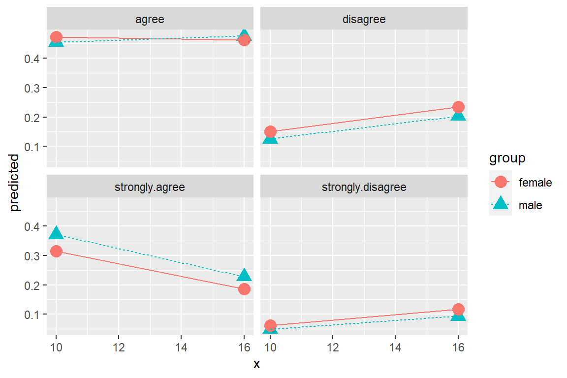
These residuals do NOT look good, especially the Q-Q plot for normality.
14.3.2.7 Marginal Plot
# A tibble: 2 x 8
   vars     n  mean    sd   min   max range     se
  <int> <dbl> <dbl> <dbl> <dbl> <dbl> <dbl>  <dbl>
1     1  2894 13.4   2.93     0    20    20 0.0544
2 2 1947 9.86 2.99 1 12 11 0.0677 educate income
Min. : 0.00 Min. : 1.000
1st Qu.:12.00 1st Qu.: 9.000
Median :13.00 Median :11.000
Mean :13.36 Mean : 9.862
3rd Qu.:16.00 3rd Qu.:12.000
Max. :20.00 Max. :12.000
NA's :9 NA's :956 ggeffects::ggemmeans(model = glm_possion_2,
terms = "educate",
condition = c(female = "male",
nonwhite = "white")) %>%
data.frame %>%
ggplot(aes(x = x,
y = predicted)) +
geom_line() +
labs(x = "Years of Formal Education",
y = "Predicted Number of Volunteer Activities")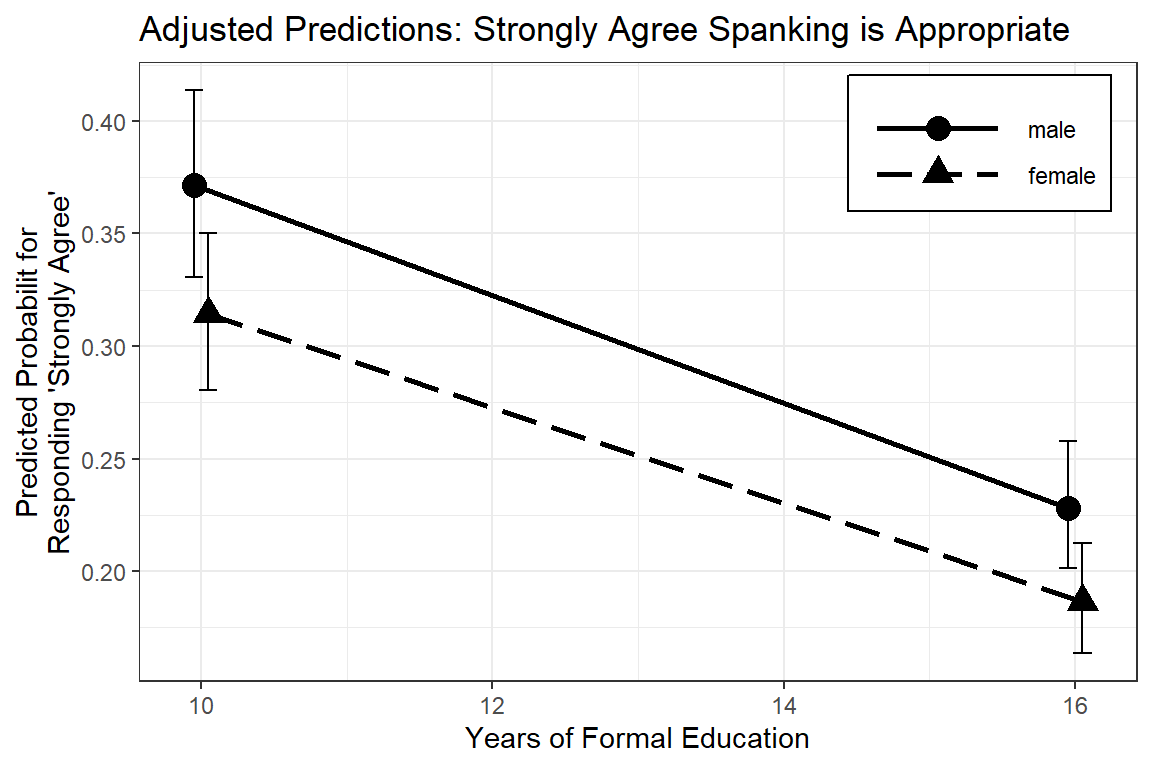
Figure 14.1: Hoffmann’s Figure 6.5
effects::Effect(focal.predictors = c("female", "nonwhite", "educate", "income"),
                mod = glm_possion_2,
                xlevels = list(educate = seq(from = 0, to = 20, by = .1),
                               income  = c(8, 10, 12))) %>%
  data.frame() %>%
  dplyr::mutate(income = factor(income) %>%
                  forcats::fct_recode("Lower Income (8)" = "8",
                                      "Middle Income (10)" = "10",
                                      "Higher Income (12)" = "12")) %>%
  ggplot(aes(x = educate,
             y = fit)) +
  geom_ribbon(aes(ymin = fit - se,  # bands = +/- 1 SEM
                  ymax = fit + se,
                  fill = female),
              alpha = .2) +
  geom_line(aes(linetype = female,
                color = female),
            size = 1) +
  theme_bw() +
  labs(x = "Education, Years",
       y = "Predicted Mean Number of Volunteer Activities",
       color = NULL,
       fill = NULL,
       linetype = NULL) +
  theme(legend.position = c(0, 1),
        legend.justification = c(-.1, 1.1),
        legend.background = element_rect(color = "black"),
        legend.key.width = unit(2, "cm")) +
  facet_grid(nonwhite ~ income)
effects::Effect(focal.predictors = c("female", "nonwhite", "educate", "income"),
                mod = glm_possion_2,
                xlevels = list(educate = seq(from = 0, to = 20, by = .1),
                               income  = c(5, 8, 12))) %>%
  data.frame() %>%
  dplyr::mutate(income = factor(income)) %>%
  ggplot(aes(x = educate,
             y = fit)) +
  geom_line(aes(linetype = fct_rev(income),
                color = fct_rev(income)),
            size = 1) +
  theme_bw() +
  labs(x = "Education, Years",
       y = "Predicted Mean Number of Volunteer Activities",
       color = "Income:",
       fill = "Income:",
       linetype = "Income:") +
  theme(legend.position = c(0, 1),
        legend.justification = c(-.1, 1.1),
        legend.background = element_rect(color = "black"),
        legend.key.width = unit(2, "cm")) +
  facet_grid(nonwhite ~ female) +
  scale_linetype_manual(values = c("solid", "longdash", "dotted"))
effects::Effect(focal.predictors = c("female", "nonwhite", "educate", "income"),
                mod = glm_possion_2,
                xlevels = list(educate = seq(from = 0, to = 20, by = .1),
                               income  = c(8, 10, 12))) %>%
  data.frame() %>%
  dplyr::mutate(income = factor(income) %>%
                  forcats::fct_recode("Lower Income (8)" = "8",
                                      "Middle Income (10)" = "10",
                                      "Higher Income (12)" = "12")) %>%
  ggplot(aes(x = educate,
             y = fit)) +
  geom_ribbon(aes(ymin = fit - se,  # bands = +/- 1 SEM
                  ymax = fit + se,
                  fill = nonwhite),
              alpha = .2) +
  geom_line(aes(linetype = nonwhite,
                color = nonwhite),
            size = 1) +
  theme_bw() +
  labs(x = "Education, Years",
       y = "Predicted Mean Number of Volunteer Activities",
       color = NULL,
       fill = NULL,
       linetype = NULL) +
  theme(legend.position = c(0, .5),
        legend.justification = c(-.05, 1.1),
        legend.background = element_rect(color = "black"),
        legend.key.width = unit(2, "cm")) +
  facet_grid(female ~ income) +
  scale_color_manual(values = c("darkgreen", "orange")) +
  scale_fill_manual(values = c("darkgreen", "orange"))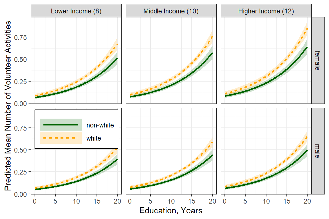
effects::Effect(focal.predictors = c("female", "educate"),
                mod = glm_possion_2,
                xlevels = list(educate = seq(from = 0,
                                             to   = 20,
                                             by = .1),
                               income = 11)) %>%          #Median Income
  data.frame() %>%
  ggplot(aes(x = educate,
             y = fit)) +
  geom_ribbon(aes(ymin = fit - se,  # bands = +/- 1 SEM
                  ymax = fit + se,
                  fill = female),
              alpha = .2) +
  geom_line(aes(linetype = female,
                color = female),
            size = 1) +
  theme_bw() +
  labs(x = "Education, Years",
       y = "Predicted Mean Number of Volunteer Activities",
       color = NULL,
       fill = NULL,
       linetype = NULL) +
  theme(legend.position = c(0, 1),
        legend.justification = c(-.1, 1.1),
        legend.background = element_rect(color = "black"),
legend.key.width = unit(2, "cm")) 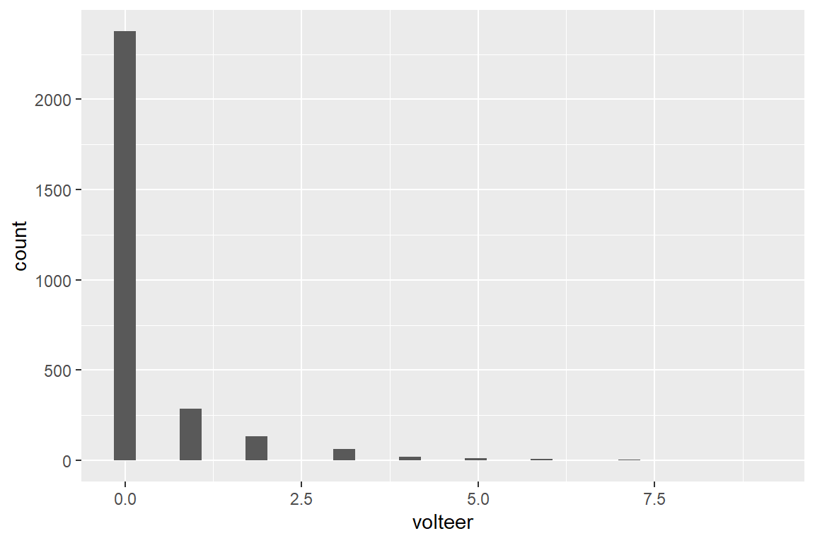
14.4 Negative Binomial Regression
14.4.1 Multiple Predictors
14.4.1.1 Fit the model
glm_negbin_1 <- MASS::glm.nb(volteer ~ female + nonwhite + educate + income,
                             data = data_gss)

summary(glm_negbin_1)
Call:
MASS::glm.nb(formula = volteer ~ female + nonwhite + educate +
    income, data = data_gss, init.theta = 0.2559648877, link = log)

Deviance Residuals:
    Min       1Q   Median       3Q      Max
-0.8798  -0.6897  -0.6141  -0.5211   2.7019

Coefficients:
                  Estimate Std. Error z value Pr(>|z|)
(Intercept)       -3.24738    0.37283  -8.710  < 2e-16 ***
femalefemale       0.28441    0.12312   2.310   0.0209 *
nonwhitenon-white -0.31107    0.16203  -1.920   0.0549 .
educate            0.11200    0.02321   4.825  1.4e-06 ***
income             0.05193    0.02264   2.293   0.0218 *
---
Signif. codes:  0 '***' 0.001 '**' 0.01 '*' 0.05 '.' 0.1 ' ' 1

(Dispersion parameter for Negative Binomial(0.256) family taken to be 1)

    Null deviance: 1068.5  on 1943  degrees of freedom
Residual deviance: 1024.3  on 1939  degrees of freedom
  (959 observations deleted due to missingness)
AIC: 2851.6

Number of Fisher Scoring iterations: 1

              Theta:  0.2560
          Std. Err.:  0.0251

 2 x log-likelihood:  -2839.5640
Note: the deviance residuals all have absolute values less than 3-4’ish…better than before
Theta in R = 1/alpha in Stata
# Hoffmann Example 6.5
texreg::knitreg(list(glm_possion_2,
                       texreghelpr::extract_glm_exp(glm_possion_2,
                                                    include.aic = FALSE,
                                                    include.bic = FALSE,
                                                    include.loglik = FALSE,
                                                    include.deviance = FALSE,
                                                    include.nobs = FALSE)),
                  custom.model.names = c("b (SE)", "IRR [95% CI]"),
                  custom.coef.map = list("(Intercept)" ="Intercept",
                                         femalefemale = "Female vs. Male",
                                         "nonwhitenon-white" = "Non-white vs. White",
                                         educate = "Education, years",
                                         income = "Income, 1000's"),
                  caption = "GLM: Multiple Possion Regression",
                  single.row = TRUE,
digits = 3)| b (SE) | IRR [95% CI] | |
|---|---|---|
| Intercept | -3.158 (0.245)*** | 0.042 [0.026; 0.068]* |
| Female vs. Male | 0.261 (0.078)*** | 1.299 [1.115; 1.513]* |
| Non-white vs. White | -0.280 (0.108)** | 0.755 [0.608; 0.930]* |
| Education, years | 0.103 (0.014)*** | 1.108 [1.077; 1.140]* |
| Income, 1000’s | 0.057 (0.016)*** | 1.058 [1.027; 1.092]* |
| AIC | 3380.860 | |
| BIC | 3408.722 | |
| Log Likelihood | -1685.430 | |
| Deviance | 2465.514 | |
| Num. obs. | 1944 | |
| p < 0.001; p < 0.01; p < 0.05 (or Null hypothesis value outside the confidence interval). | ||
14.4.1.2 Predictions
Note: These means are on the original scale (number of volunteer activities in the past year). These standard errors are called “delta-method standard errors”
effects::Effect(focal.predictors = c("female"),
                mod = glm_negbin_1,
                xlevels = list(nonwhite = "non-white",
                               educate = 5,
                               income = 12)) %>%
  data.frame()
# A tibble: 2 x 5
female fit se lower upper
<fct> <dbl> <dbl> <dbl> <dbl>
1 male 0.289 0.0257 0.243 0.344
2 female 0.384 0.0322 0.326 0.453ggeffects::ggemmeans(model = glm_negbin_1,
terms = c("female"),
condition = c(nonwhite = "white",
educate = 12,
income = 5))# A tibble: 2 x 6
x predicted std.error conf.low conf.high group
<fct> <dbl> <dbl> <dbl> <dbl> <fct>
1 male 0.193 0.157 0.142 0.263 1
2 female 0.257 0.137 0.196 0.336 1 Compare to the Poisson:
ggeffects::ggemmeans(model = glm_possion_2,
                     terms = c("female"),
                     condition = c(nonwhite = "white",
                                   educate = 12,
                                   income = 5))
# A tibble: 2 x 6
x predicted std.error conf.low conf.high group
<fct> <dbl> <dbl> <dbl> <dbl> <fct>
1 male 0.194 0.109 0.157 0.240 1
2 female 0.252 0.0952 0.209 0.303 1 Note: The predictions are very similar for Poisson and Negative Binomial…therefor the overdisperssion does not affect the sex difference much, but it may affect other things…
14.4.1.3 Parameter Estimates
Coefficients are in terms of the LOG of the number of times a person volunteers per year.
      (Intercept)      femalefemale nonwhitenon-white           educate
      -3.24738340        0.28440826       -0.31107286        0.11199528
           income
       0.05193102
Exponentiating the coefficients (betas) returns the values to the original scale (number of times a person volunteers per year) and is refered to as the incident rate ratio IRR.
      (Intercept)      femalefemale nonwhitenon-white           educate
        0.0388758         1.3289754         0.7326605         1.1185076
           income
1.0533031 texreg::knitreg(list(glm_negbin_1,
texreghelpr::extract_glm_exp(glm_negbin_1,
include.aic = FALSE,
include.bic = FALSE,
include.loglik = FALSE,
include.deviance = FALSE,
include.nobs = FALSE)),
custom.model.names = c("b (SE)", "IRR [95% CI]"),
custom.coef.map = list("(Intercept)" ="Intercept",
femalefemale = "Female vs. Male",
"nonwhitenon-white" = "Non-white vs. White",
educate = "Education, Years",
income = "Income"),
caption = "GLM: Negitive Binomial Regression",
single.row = TRUE,
digits = 3)| b (SE) | IRR [95% CI] | |
|---|---|---|
| Intercept | -3.247 (0.373)*** | 0.039 [0.018; 0.081]* |
| Female vs. Male | 0.284 (0.123)* | 1.329 [1.043; 1.696]* |
| Non-white vs. White | -0.311 (0.162) | 0.733 [0.533; 1.008]* |
| Education, Years | 0.112 (0.023)*** | 1.119 [1.067; 1.173]* |
| Income | 0.052 (0.023)* | 1.053 [1.008; 1.101]* |
| AIC | 2851.564 | |
| BIC | 2884.999 | |
| Log Likelihood | -1419.782 | |
| Deviance | 1024.343 | |
| Num. obs. | 1944 | |
| p < 0.001; p < 0.01; p < 0.05 (or Null hypothesis value outside the confidence interval). | ||
14.4.1.4 Residual Diagnostics
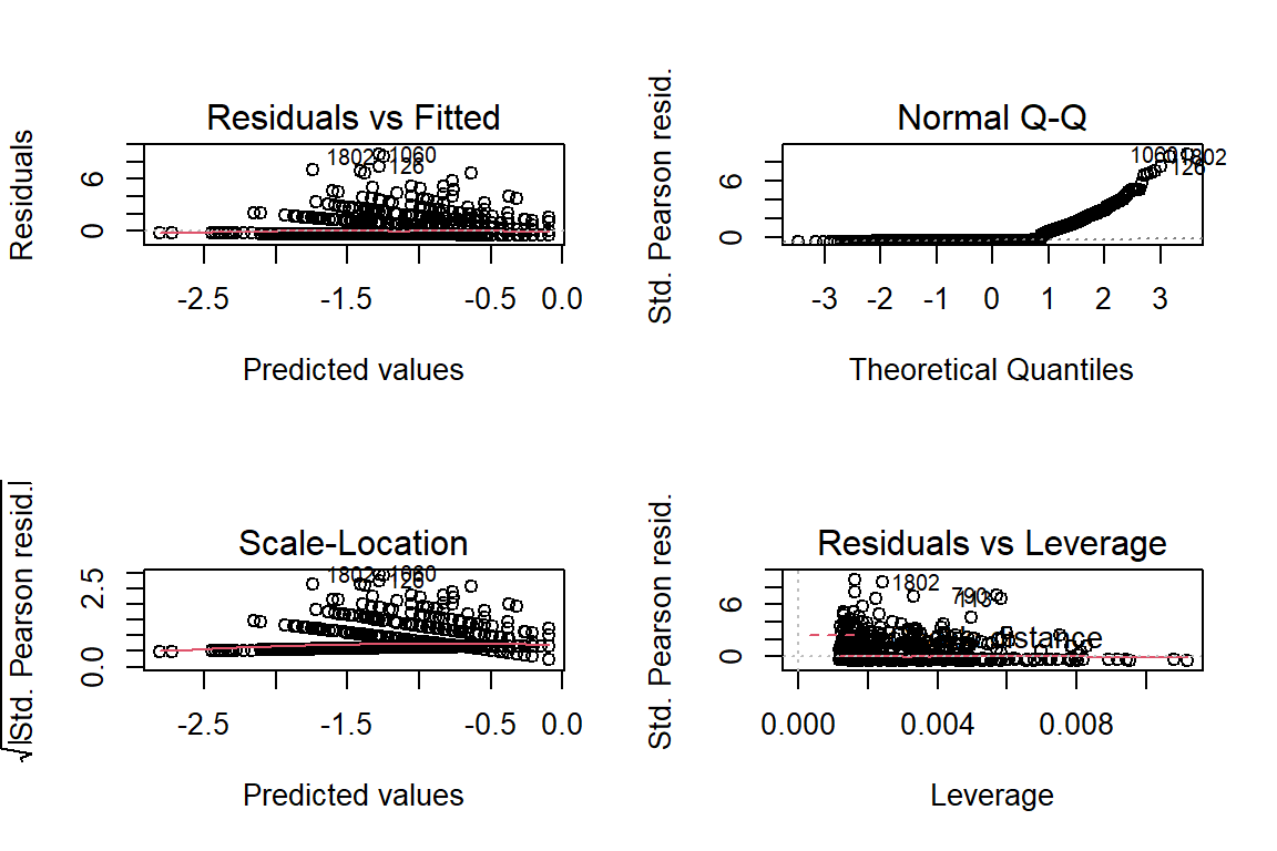
These still don’t look very good :(
14.4.1.5 Compare models
# A tibble: 2 x 10
  Model Type    AIC   BIC R2_Nagelkerke  RMSE SCORE_LOG SCORE_SPHERICAL       BF
  <chr> <chr> <dbl> <dbl>         <dbl> <dbl>     <dbl>           <dbl>    <dbl>
1 glm_~ negb~ 2852. 2885.        0.0531 0.726    -0.808          0.0210 5.31e113
2 glm_~ glm   3381. 3409.        0.0693 1.13     -0.867          0.0210 1.00e  0
# ... with 1 more variable: Performance_Score <dbl>
14.5 Zero Inflated Poisson
14.5.0.1 Fit the model
glm_zip_1 <- pscl::zeroinfl(volteer ~ female + nonwhite + educate + income | educate,
                               data = data_gss)

summary(glm_zip_1)
Call:
pscl::zeroinfl(formula = volteer ~ female + nonwhite + educate + income |
    educate, data = data_gss)

Pearson residuals:
    Min      1Q  Median      3Q     Max
-0.5778 -0.4416 -0.3908 -0.3382  9.4776

Count model coefficients (poisson with log link):
                  Estimate Std. Error z value Pr(>|z|)
(Intercept)       -1.09676    0.34808  -3.151  0.00163 **
femalefemale       0.20623    0.09452   2.182  0.02912 *
nonwhitenon-white -0.20099    0.13444  -1.495  0.13491
educate            0.05649    0.02140   2.639  0.00832 **
income             0.04888    0.01882   2.597  0.00940 **

Zero-inflation model coefficients (binomial with logit link):
            Estimate Std. Error z value Pr(>|z|)
(Intercept)  2.01175    0.41193   4.884 1.04e-06 ***
educate     -0.07180    0.02769  -2.594   0.0095 **
---
Signif. codes:  0 '***' 0.001 '**' 0.01 '*' 0.05 '.' 0.1 ' ' 1

Number of iterations in BFGS optimization: 12
Log-likelihood: -1434 on 7 Df count_(Intercept) count_femalefemale count_nonwhitenon-white
0.3339504 1.2290310 0.8179193
count_educate count_income zero_(Intercept)
1.0581113 1.0500956 7.4763533
zero_educate
0.9307151 Compares two models fit to the same data that do not nest via Vuong’s non-nested test.
Vuong Non-Nested Hypothesis Test-Statistic:
(test-statistic is asymptotically distributed N(0,1) under the
 null that the models are indistinguishible)
-------------------------------------------------------------
              Vuong z-statistic             H_A    p-value
Raw                    8.000316 model1 > model2 6.6613e-16
AIC-corrected          7.936582 model1 > model2 9.9920e-16
BIC-corrected          7.759003 model1 > model2 4.3299e-15
14.6 Zero Inflated Negative Binomial
14.6.0.1 Fit the model
glm_zinb_1 <- pscl::zeroinfl(volteer ~ female + nonwhite + educate + income | educate,
                               data = data_gss,
                             dist = "negbin")

summary(glm_zinb_1)
Call:
pscl::zeroinfl(formula = volteer ~ female + nonwhite + educate + income |
    educate, data = data_gss, dist = "negbin")

Pearson residuals:
    Min      1Q  Median      3Q     Max
-0.5146 -0.4122 -0.3704 -0.3222  8.8088

Count model coefficients (negbin with log link):
                  Estimate Std. Error z value Pr(>|z|)
(Intercept)       -1.79283    0.54745  -3.275  0.00106 **
femalefemale       0.26245    0.11745   2.235  0.02544 *
nonwhitenon-white -0.28519    0.15603  -1.828  0.06758 .
educate            0.06817    0.03317   2.055  0.03986 *
income             0.05292    0.02159   2.451  0.01426 *
Log(theta)         0.05055    0.46241   0.109  0.91295

Zero-inflation model coefficients (binomial with logit link):
            Estimate Std. Error z value Pr(>|z|)
(Intercept)  1.28315    0.71437   1.796   0.0725 .
educate     -0.07208    0.04684  -1.539   0.1239
---
Signif. codes:  0 '***' 0.001 '**' 0.01 '*' 0.05 '.' 0.1 ' ' 1

Theta = 1.0518
Number of iterations in BFGS optimization: 27
Log-likelihood: -1416 on 8 Df count_(Intercept) count_femalefemale count_nonwhitenon-white
0.1664876 1.3001178 0.7518694
count_educate count_income zero_(Intercept)
1.0705453 1.0543420 3.6079992
zero_educate
0.9304589 Vuong Non-Nested Hypothesis Test-Statistic:
(test-statistic is asymptotically distributed N(0,1) under the
null that the models are indistinguishible)
-------------------------------------------------------------
Vuong z-statistic H_A p-value
Raw 1.3486684 model1 > model2 0.088722
AIC-corrected 0.5592184 model1 > model2 0.288006
BIC-corrected -1.6403877 model2 > model1 0.050462Vuong Non-Nested Hypothesis Test-Statistic:
(test-statistic is asymptotically distributed N(0,1) under the
null that the models are indistinguishible)
-------------------------------------------------------------
Vuong z-statistic H_A p-value
Raw -2.428631 model2 > model1 0.007578
AIC-corrected -2.428631 model2 > model1 0.007578
BIC-corrected -2.428631 model2 > model1 0.007578The ‘best’ model is the zero-inflated negative binomial