6 Interactions Example
library(tidyverse)
library(emmeans)
library(furniture)
library(stargazer)
library(psych)
library(texreg)
library(interactions)
Taken from: https://stats.idre.ucla.edu/r/seminars/interactions-r/
6.1 Motivation
Suppose you are doing a simple study on weight loss and notice that people who spend more time exercising lose more weight. Upon further analysis you notice that those who spend the same amount of time exercising lose more weight if they are more effortful. The more effort people put into their workouts, the less time they need to spend exercising. This is popular in workouts like high intensity interval training (HIIT).
You know that hours spent exercising improves weight loss, but how does it interact with effort? Here are three questions you can ask based on hypothetical scenarios.
I’m just starting out and don’t want to put in too much effort. How many hours per week of exercise do I need to put in to lose 5 pounds?
I’m moderately fit and can put in an average level of effort into my workout. For every one hour increase per week in exercise, how much additional weight loss do I expect?
I’m a crossfit athlete and can perform with the utmost intensity. How much more weight loss would I expect for every one hour increase in exercise compared to the average amount of effort most people put in?
Additionally, we can visualize the interaction to help us understand these relationships.
6.2 The Weight Loss Study
This is a hypothetical study of weight loss for 900 participants in a year-long study of 3 different exercise programs, a jogging program, a swimming program, and a reading program which serves as a control activity.
Variables
loss: weight loss (continuous), positive = weight loss, negative scores = weight gainhours: hours spent exercising (continuous)effort: effort during exercise (continuous)- 0 = minimal physical effort and
- 50 = maximum effort
prog: exercise program (categorical)- jogging=1
- swimming=2
- reading=3
gender: participant gender (binary)- male=1
- female=2
Definitions
What exactly do I mean by decomposing, probing, and plotting an interaction?
- decompose: to break down the interaction into its lower order components (i.e., predicted means or simple slopes)
- probe: to use hypothesis testing to assess the statistical significance of simple slopes and simple slope differences (i.e., interactions)
- plot: to visually display the interaction in the form of simple slopes such as values of the dependent variable are on the y-axis, values of the predictor is on the x-axis, and the moderator separates the lines or bar graphs
Let’s define the essential elements of the interaction in a regression:
- DV: dependent variable (Y), the outcome of your study (e.g., weight loss)
- IV: independent variable (X), the predictor of your outcome (e.g., time exercising)
- MV: moderating variable (W) or moderator, a predictor that changes the relationship of the IV on the DV (e.g, effort)
- coefficient: estimate of the direction and magnitude of the relationship between an IV and DV
- continuous variable: a variable that can be measured on a continuous scale, e.g., weight, height
- categorical or binary variable: a variable that takes on discrete values, binary variables take on exactly two values, categorical variables can take on 3 or more values (e.g., gender, ethnicity)
- main effects or slopes: effects or slopes for models that do not involve interaction terms
- simple slope: when a continuous IV interacts with an MV, its slope at a particular level of an MV
- simple effect: when a categorical IV interacts with an MV, its effect at a particular level of an MV
6.2.1 Import Data
data_raw <- read.csv("https://stats.idre.ucla.edu/wp-content/uploads/2019/03/exercise.csv")tibble::glimpse(data_raw)Rows: 900
Columns: 6
$ id <int> 1, 2, 3, 4, 5, 6, 7, 8, 9, 10, 11, 12, 13, 14, 15, 16, 17, 18, ~
$ loss <dbl> 18.022263, 10.186416, 19.747276, 1.883600, 14.242589, 19.694731~
$ hours <dbl> 1.836704, 2.389360, 2.362117, 2.520866, 1.889828, 2.367162, 1.9~
$ effort <dbl> 37.71218, 26.72401, 36.31657, 20.70048, 24.72712, 33.66948, 31.~
$ gender <int> 1, 1, 1, 1, 1, 1, 1, 1, 1, 1, 1, 1, 1, 1, 1, 1, 1, 1, 1, 1, 1, ~
$ prog <int> 1, 1, 1, 1, 1, 1, 1, 1, 1, 1, 1, 1, 1, 1, 1, 1, 1, 1, 1, 1, 1, ~data_raw %>%
summary() id loss hours effort
Min. : 1.0 Min. :-17.138 Min. :0.1751 Min. :12.95
1st Qu.:225.8 1st Qu.: -1.743 1st Qu.:1.6764 1st Qu.:26.26
Median :450.5 Median : 7.883 Median :2.0051 Median :29.63
Mean :450.5 Mean : 10.021 Mean :2.0024 Mean :29.66
3rd Qu.:675.2 3rd Qu.: 20.049 3rd Qu.:2.3375 3rd Qu.:33.10
Max. :900.0 Max. : 54.150 Max. :4.0722 Max. :44.08
gender prog
Min. :1.0 Min. :1
1st Qu.:1.0 1st Qu.:1
Median :1.5 Median :2
Mean :1.5 Mean :2
3rd Qu.:2.0 3rd Qu.:3
Max. :2.0 Max. :3 6.2.2 Wrangle the data
data_clean <- data_raw %>%
  dplyr::mutate(id = factor(id)) %>%
  dplyr::mutate(gender = factor(gender) %>%
                  forcats::fct_recode("Male"   = "1",
                                      "Female" = "2")) %>%
  dplyr::mutate(prog = factor(prog) %>%
                  forcats::fct_recode("Jog"  = "1",
                                      "Swim" = "2",
"Read" = "3"))tibble::glimpse(data_clean)Rows: 900
Columns: 6
$ id <fct> 1, 2, 3, 4, 5, 6, 7, 8, 9, 10, 11, 12, 13, 14, 15, 16, 17, 18, ~
$ loss <dbl> 18.022263, 10.186416, 19.747276, 1.883600, 14.242589, 19.694731~
$ hours <dbl> 1.836704, 2.389360, 2.362117, 2.520866, 1.889828, 2.367162, 1.9~
$ effort <dbl> 37.71218, 26.72401, 36.31657, 20.70048, 24.72712, 33.66948, 31.~
$ gender <fct> Male, Male, Male, Male, Male, Male, Male, Male, Male, Male, Mal~
$ prog <fct> Jog, Jog, Jog, Jog, Jog, Jog, Jog, Jog, Jog, Jog, Jog, Jog, Jog~summary(data_clean) id loss hours effort gender
1 : 1 Min. :-17.138 Min. :0.1751 Min. :12.95 Male :450
2 : 1 1st Qu.: -1.743 1st Qu.:1.6764 1st Qu.:26.26 Female:450
3 : 1 Median : 7.883 Median :2.0051 Median :29.63
4 : 1 Mean : 10.021 Mean :2.0024 Mean :29.66
5 : 1 3rd Qu.: 20.049 3rd Qu.:2.3375 3rd Qu.:33.10
6 : 1 Max. : 54.150 Max. :4.0722 Max. :44.08
(Other):894
prog
Jog :300
Swim:300
Read:300
6.3 Exploratory Data Analysis
6.3.1 Summary Statistics
data_clean %>%
  psych::describe()
# A tibble: 6 x 13
vars n mean sd median trimmed mad min max range
<int> <dbl> <dbl> <dbl> <dbl> <dbl> <dbl> <dbl> <dbl> <dbl>
1 1 900 450. 260. 450. 450. 334. 1 900 899
2 2 900 10.0 14.1 7.88 9.06 15.4 -17.1 54.2 71.3
3 3 900 2.00 0.495 2.01 2.00 0.492 0.175 4.07 3.90
4 4 900 29.7 5.14 29.6 29.6 5.08 12.9 44.1 31.1
5 5 900 1.5 0.500 1.5 1.5 0.741 1 2 1
6 6 900 2 0.817 2 2 1.48 1 3 2
# ... with 3 more variables: skew <dbl>, kurtosis <dbl>, se <dbl>data_clean %>%
stargazer::stargazer(type = "text")
==============================================================
Statistic  N   Mean  St. Dev.   Min   Pctl(25) Pctl(75)  Max
--------------------------------------------------------------
loss      900 10.021  14.100  -17.138  -1.743   20.049  54.150
hours     900 2.002   0.495    0.175   1.676    2.337   4.072
effort    900 29.659  5.143   12.949   26.258   33.095  44.076
--------------------------------------------------------------
data_clean %>%
furniture::table1(gender, loss, hours, effort)
-----------------------------
           Mean/Count (SD/%)
           n = 900
 gender
    Male   450 (50%)
    Female 450 (50%)
 loss
           10.0 (14.1)
 hours
           2.0 (0.5)
 effort
           29.7 (5.1)
-----------------------------
data_clean %>%
dplyr::group_by(prog) %>%
furniture::table1("Gender" = gender,
"Weight Loss, pounds" = loss,
"Time Spent in Program, hours" = hours,
"Effort in Program" = effort,
digits = 2,
output = "markdown",
total = TRUE,
test = TRUE)| Total | Jog | Swim | Read | P-Value | |
|---|---|---|---|---|---|
| n = 900 | n = 300 | n = 300 | n = 300 | ||
| Gender | 1 | ||||
| Male | 450 (50%) | 150 (50%) | 150 (50%) | 150 (50%) | |
| Female | 450 (50%) | 150 (50%) | 150 (50%) | 150 (50%) | |
| Weight Loss, pounds | <.001 | ||||
| 10.02 (14.10) | 8.03 (7.45) | 25.82 (8.92) | -3.79 (4.11) | ||
| Time Spent in Program, hours | 0.469 | ||||
| 2.00 (0.49) | 1.99 (0.47) | 1.99 (0.48) | 2.03 (0.53) | ||
| Effort in Program | 0.18 | ||||
| 29.66 (5.14) | 30.05 (5.04) | 29.65 (5.17) | 29.28 (5.20) |
6.3.2 Correlations
data_clean %>%
  dplyr::select_if(is.numeric) %>%
  furniture::tableC()
---------------------------------------------
           [1]           [2]           [3]
 [1]loss   1.00
 [2]hours  0.087 (0.009) 1.00
 [3]effort 0.259 (<.001) 0.016 (0.626) 1.00
---------------------------------------------
data_clean %>%
cor.test(~ loss + hours,
data = .)
    Pearson's product-moment correlation

data:  loss and hours
t = 2.6054, df = 898, p-value = 0.009329
alternative hypothesis: true correlation is not equal to 0
95 percent confidence interval:
 0.02138902 0.15110872
sample estimates:
       cor
0.08661599
data_clean %>%
cor.test(~ loss + effort,
data = .)
    Pearson's product-moment correlation

data:  loss and effort
t = 8.0213, df = 898, p-value = 3.255e-15
alternative hypothesis: true correlation is not equal to 0
95 percent confidence interval:
 0.1965432 0.3185360
sample estimates:
      cor
0.2585703
data_clean %>%
cor.test(~ hours + effort,
data = .)
    Pearson's product-moment correlation

data:  hours and effort
t = 0.48812, df = 898, p-value = 0.6256
alternative hypothesis: true correlation is not equal to 0
95 percent confidence interval:
 -0.04911364  0.08154791
sample estimates:
       cor
0.01628667
data_clean %>%
dplyr::select_if(is.numeric) %>%
cor() loss hours effort
loss 1.00000000 0.08661599 0.25857026
hours 0.08661599 1.00000000 0.01628667
effort 0.25857026 0.01628667 1.00000000data_clean %>%
dplyr::select_if(is.numeric) %>%
cor() %>%
corrplot::corrplot()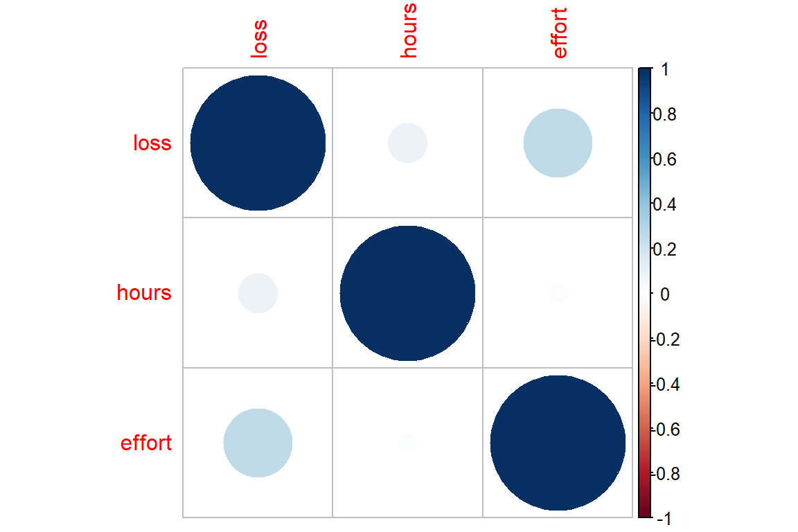
data_clean %>%
  dplyr::select_if(is.numeric) %>%
cor() %>%
corrplot::corrplot.mixed()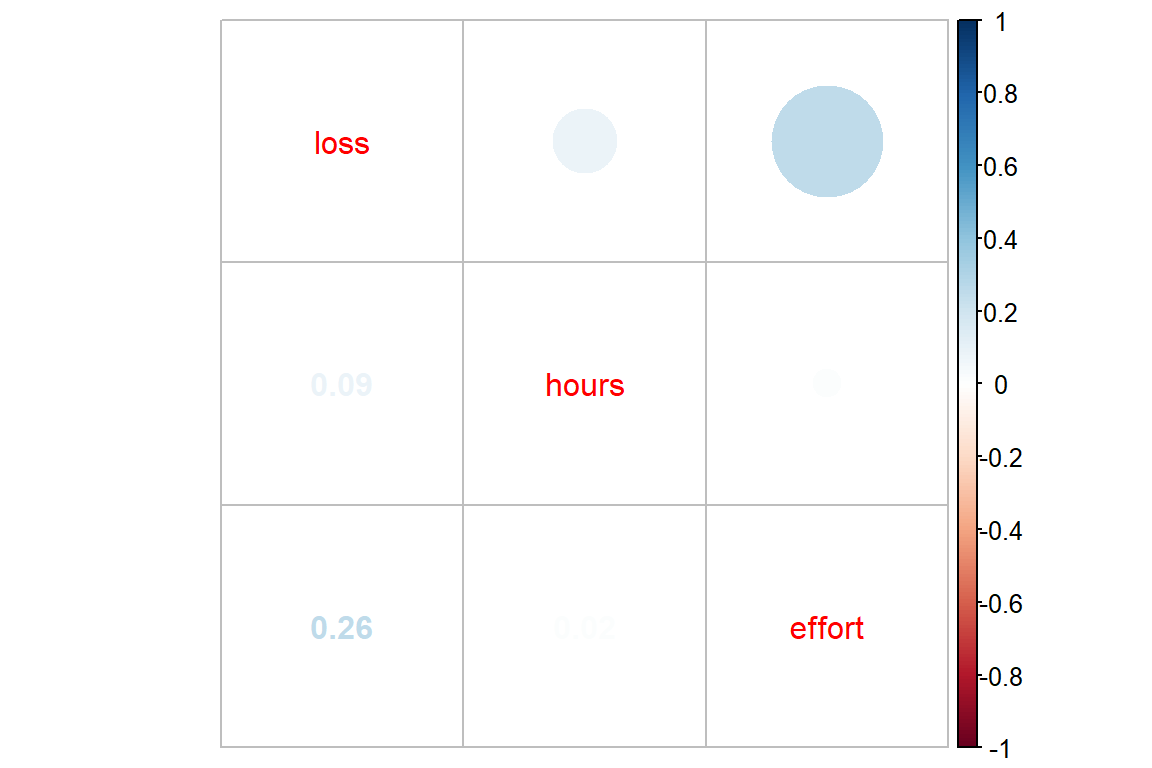
6.3.3 Visualization Bivariate Relationships
data_clean %>%
  ggplot(aes(x = hours,
             y = loss)) +
  geom_point() +
  theme_bw()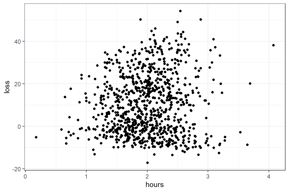
data_clean %>%
  ggplot(aes(x = hours,
             y = loss)) +
  geom_point() +
  geom_smooth(method = "lm") +
  theme_bw()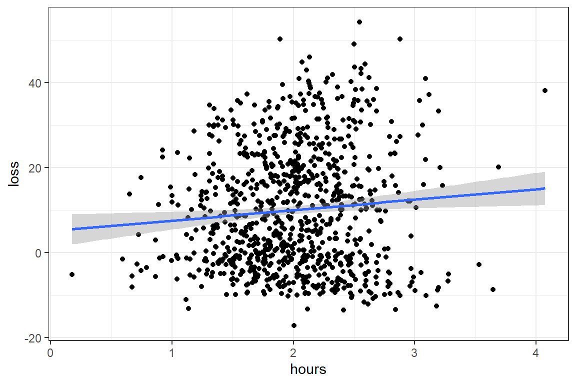
data_clean %>%
  ggplot(aes(x = hours,
             y = loss)) +
  geom_point() +
  geom_smooth(method = "lm") +
  theme_bw() +
  facet_grid(~ gender)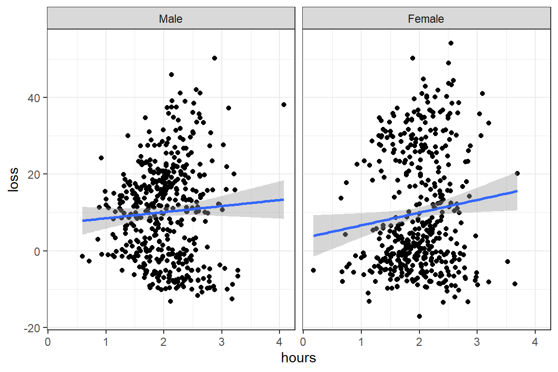
data_clean %>%
  ggplot(aes(x = hours,
             y = loss)) +
  geom_point() +
  geom_smooth(method = "lm") +
  theme_bw() +
  facet_grid(~ prog)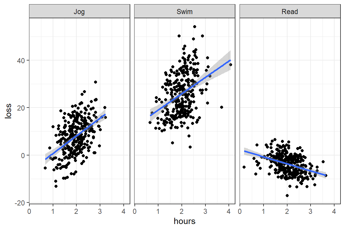
data_clean %>%
  ggplot(aes(x = hours,
             y = loss)) +
  geom_point() +
  geom_smooth(method = "lm") +
  theme_bw() +
  facet_grid(gender ~ prog)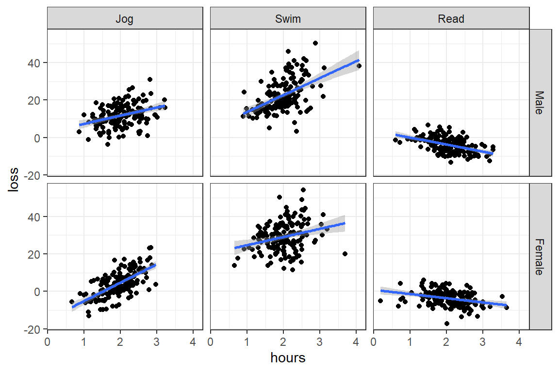
6.4 Simple Linear Regression
6.4.1 Fit a MLR Model
Question: Does time spent on a program effect weight loss?
fit_lm_loss_hr <- lm(loss ~ hours,        # DV ~ IV's
data = data_clean)summary(fit_lm_loss_hr)
Call:
lm(formula = loss ~ hours, data = data_clean)

Residuals:
    Min      1Q  Median      3Q     Max
-27.164 -11.388  -2.086  10.011  42.787

Coefficients:
            Estimate Std. Error t value Pr(>|t|)
(Intercept)   5.0757     1.9550   2.596  0.00958 **
hours         2.4696     0.9479   2.605  0.00933 **
---
Signif. codes:  0 '***' 0.001 '**' 0.01 '*' 0.05 '.' 0.1 ' ' 1

Residual standard error: 14.06 on 898 degrees of freedom
Multiple R-squared:  0.007502,  Adjusted R-squared:  0.006397
F-statistic: 6.788 on 1 and 898 DF,  p-value: 0.009329
Answer: Yes. There is evidence that an additional hour in a program is associated with slightly more weight lost, b = 2.47, p = .009, R^2 < .01.
6.4.2 Check Assumptions
Base function to plot main residual diagnostics to asses assumptions
http://www.contrib.andrew.cmu.edu/~achoulde/94842/homework/regression_diagnostics.html
https://daviddalpiaz.github.io/appliedstats/model-diagnostics.html
par(mfrow = c(2, 2))   # sets up a 2x2 grid of plots in base R
plot(fit_lm_loss_hr)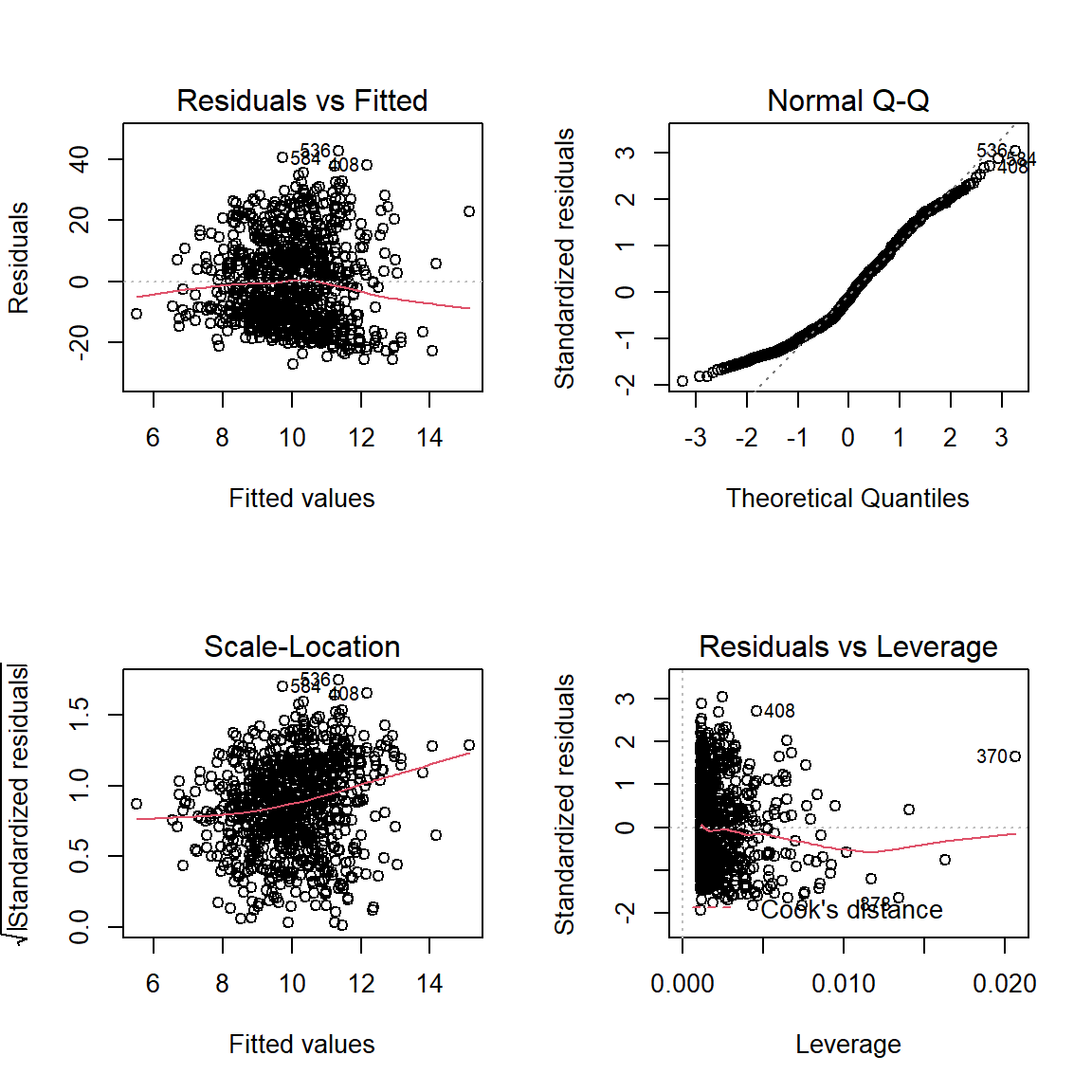
par(mfrow = c(1, 1)) # make sure to return back to a single plotfit_lm_loss_hr %>%
car::residualPlot(type = "rstandard")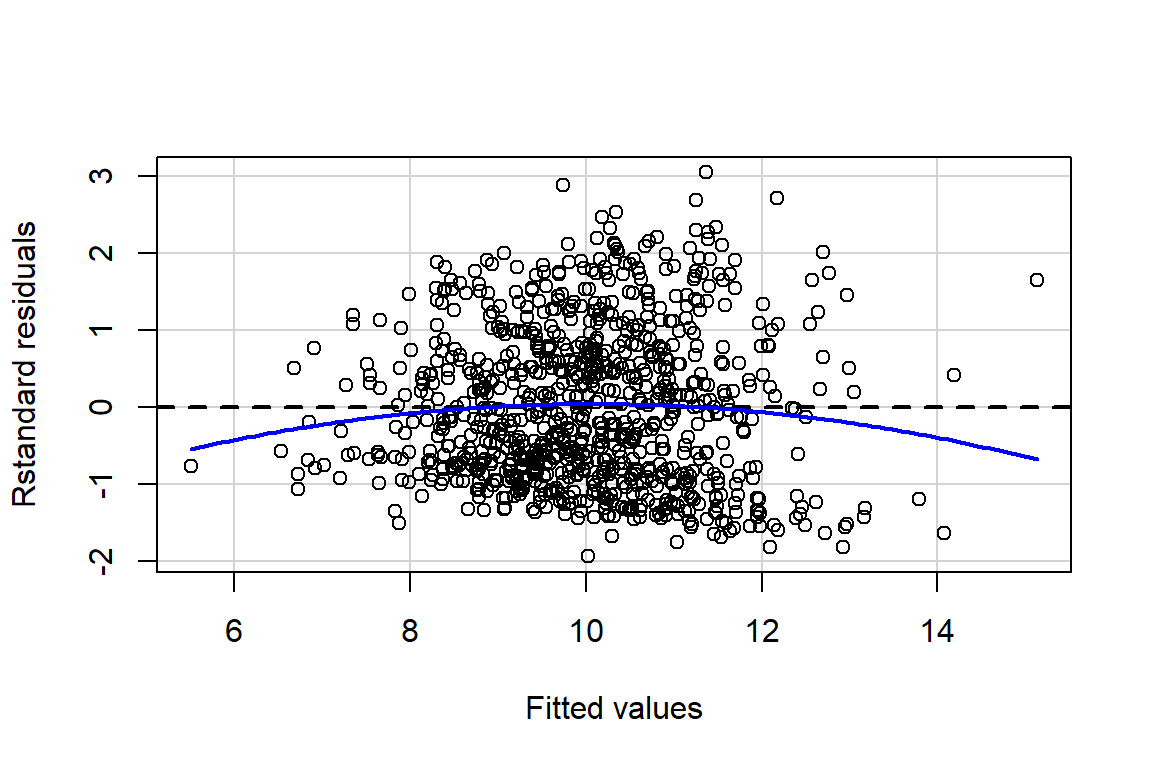
car::qqPlot(residuals(fit_lm_loss_hr))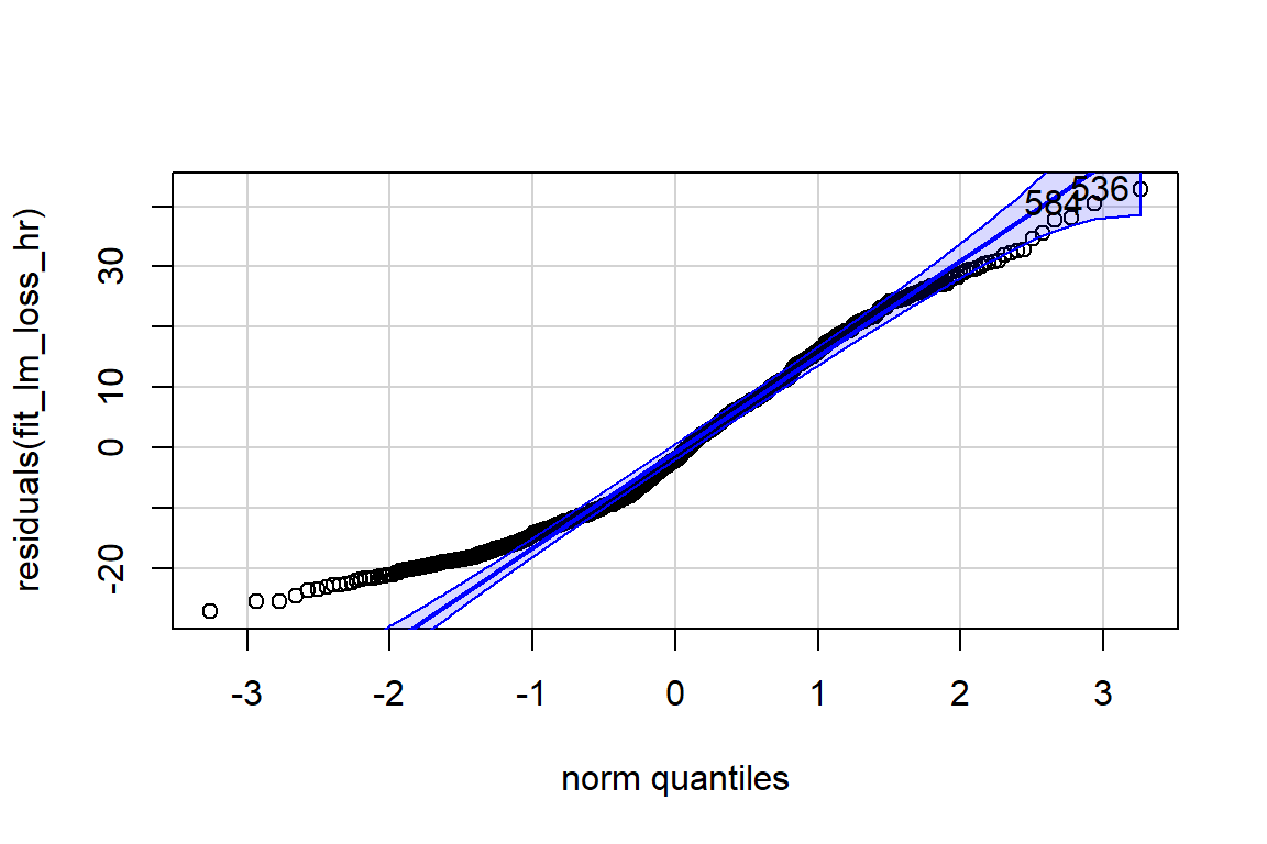
[1] 536 5846.4.3 Predict and Pariwise Tests
fit_lm_loss_hr %>%
  emmeans::emmeans(~ hours)   # default for mean hours
hours emmean SE df lower.CL upper.CL
2 10 0.469 898 9.1 10.9
Confidence level used: 0.95 Interpretation: A participant that spends 2 hours on their program looses 10 pounds on average, SE = 0.47, 95% CI [9.1, 10.9].
fit_lm_loss_hr %>%
  emmeans::emmeans(~ hours,
                   at = list(hours = 1:4))  # set hours to plug in
hours emmean SE df lower.CL upper.CL
1 7.55 1.059 898 5.47 9.62
2 10.01 0.469 898 9.10 10.93
3 12.48 1.055 898 10.41 14.56
4 14.95 1.951 898 11.13 18.78
Confidence level used: 0.95 Interpretation: Overall, on average the effect of time is an additional 2.47 pounds lost per hour spent on a program.
6.4.4 Plot Estimated Marginal Means
create a sequence of numbers
seq(from = .25, to = 4, by = .25) [1] 0.25 0.50 0.75 1.00 1.25 1.50 1.75 2.00 2.25 2.50 2.75 3.00 3.25 3.50 3.75
[16] 4.00fit_lm_loss_hr %>%
emmeans::emmeans(~ hours,
at = list(hours = seq(from = .25, to = 4, by = .25))) %>%
data.frame()# A tibble: 16 x 6
hours emmean SE df lower.CL upper.CL
<dbl> <dbl> <dbl> <dbl> <dbl> <dbl>
1 0.25 5.69 1.73 898 2.31 9.08
2 0.5 6.31 1.50 898 3.37 9.25
3 0.75 6.93 1.28 898 4.42 9.43
4 1 7.55 1.06 898 5.47 9.62
5 1.25 8.16 0.853 898 6.49 9.84
6 1.5 8.78 0.668 898 7.47 10.1
7 1.75 9.40 0.526 898 8.37 10.4
8 2 10.0 0.469 898 9.10 10.9
9 2.25 10.6 0.524 898 9.60 11.7
10 2.5 11.2 0.665 898 9.94 12.6
11 2.75 11.9 0.850 898 10.2 13.5
12 3 12.5 1.06 898 10.4 14.6
13 3.25 13.1 1.27 898 10.6 15.6
14 3.5 13.7 1.49 898 10.8 16.7
15 3.75 14.3 1.72 898 11.0 17.7
16 4 15.0 1.95 898 11.1 18.8 fit_lm_loss_hr %>%
emmeans::emmeans(~ hours,
at = list(hours = seq(from = .25, to = 4, by = .25))) %>%
data.frame() %>%
ggplot(aes(x = hours,
y = emmean)) +
geom_ribbon(aes(ymin = lower.CL,
ymax = upper.CL),
alpha = .25) +
geom_line() +
theme_bw()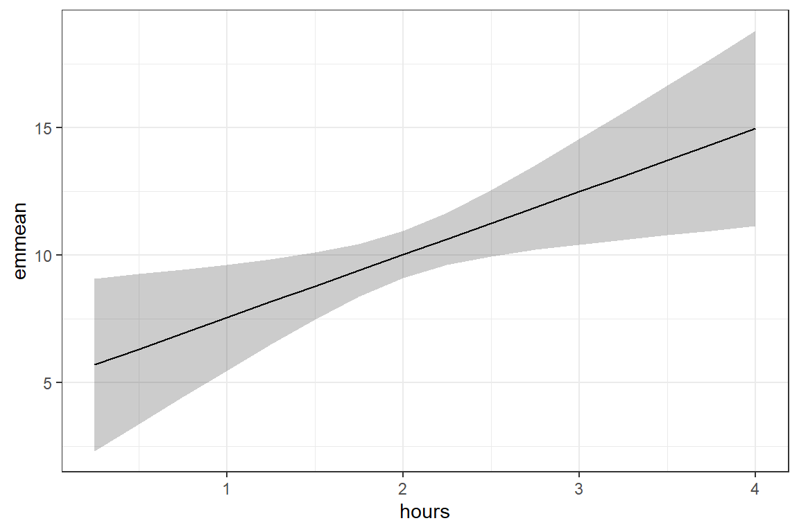
6.5 Continuous by Continuous
6.5.1 Fit MLR Model
The same model:
* loss ~ hours*effort
* loss ~ hours + effore + hours:effort
Question: Is there an interaction between time spent and effort in a weight loss program?
fit_lm_loss_hr_eff <- lm(loss ~ hours*effort,
data = data_clean)summary(fit_lm_loss_hr_eff)
Call:
lm(formula = loss ~ hours * effort, data = data_clean)

Residuals:
   Min     1Q Median     3Q    Max
-29.52 -10.60  -1.78  11.13  34.51

Coefficients:
             Estimate Std. Error t value Pr(>|t|)
(Intercept)   7.79864   11.60362   0.672   0.5017
hours        -9.37568    5.66392  -1.655   0.0982 .
effort       -0.08028    0.38465  -0.209   0.8347
hours:effort  0.39335    0.18750   2.098   0.0362 *
---
Signif. codes:  0 '***' 0.001 '**' 0.01 '*' 0.05 '.' 0.1 ' ' 1

Residual standard error: 13.56 on 896 degrees of freedom
Multiple R-squared:  0.07818,   Adjusted R-squared:  0.07509
F-statistic: 25.33 on 3 and 896 DF,  p-value: 9.826e-16
Answer: Effect does moderate time spent in a program for weight loss, b = 0.39, p = .036. The combined effect of time and effort account for nearly 8% of the variation in pounds lost.
6.5.2 Table of Parameter Estimates
Sometimes its nice to have a table of the parameter estimates of competing models.
texreg::screenreg(list(fit_lm_loss_hr,
                       fit_lm_loss_hr_eff),
                  single.row = TRUE)
================================================
              Model 1           Model 2
------------------------------------------------
(Intercept)     5.08 (1.96) **    7.80 (11.60)
hours           2.47 (0.95) **   -9.38  (5.66)
effort                           -0.08  (0.38)
hours:effort                      0.39  (0.19) *
------------------------------------------------
R^2             0.01              0.08
Adj. R^2        0.01              0.08
Num. obs.     900               900
================================================
*** p < 0.001; ** p < 0.01; * p < 0.05
6.5.3 Check Assumptions
par(mfrow = c(2, 2))
plot(fit_lm_loss_hr_eff)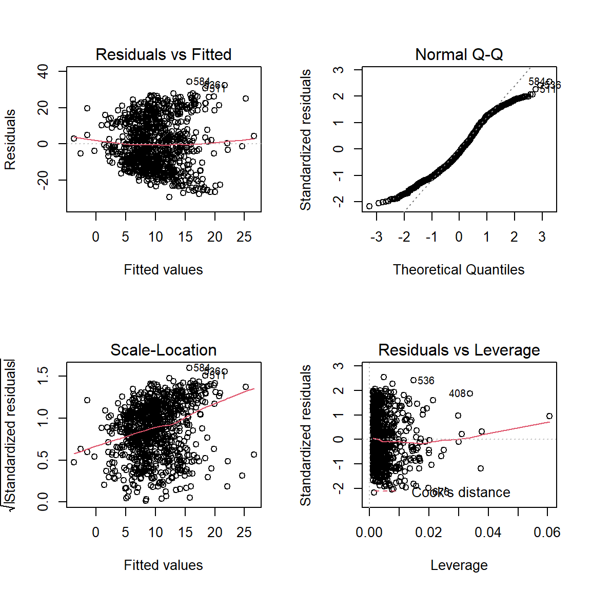
par(mfrow = c(1, 1))6.5.4 Plot Estimated Marginal Means
The emmeans package can make interaction plots with the emmip() function, but it only can create confidene intervals, not confidence bands.
fit_lm_loss_hr_eff %>%
  emmeans::emmip(effort ~ hours,
                 at = list(hours = seq(from = .25, to = 4, by = .25),
                           effort = c(20, 30, 40)),
                 CIs = TRUE)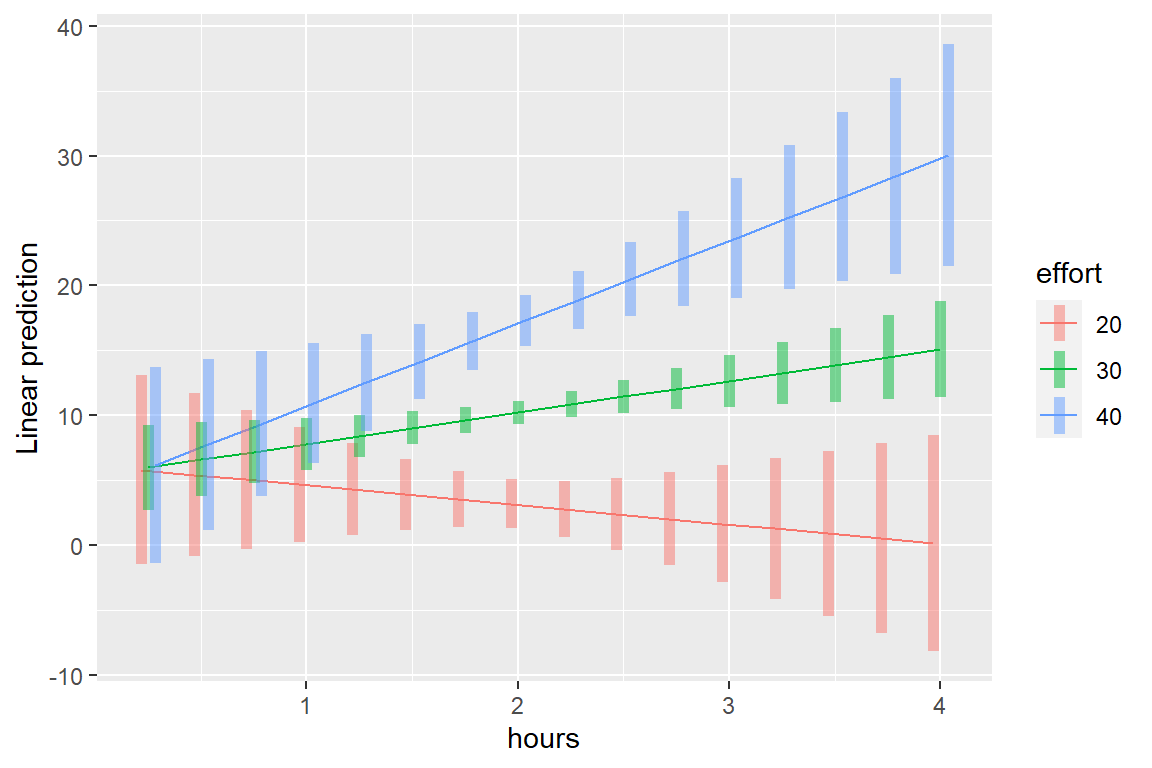
fit_lm_loss_hr_eff %>%
  interactions::interact_plot(pred = hours,
                              modx = effort,
                              interval = TRUE,
                              int.type = "confidence")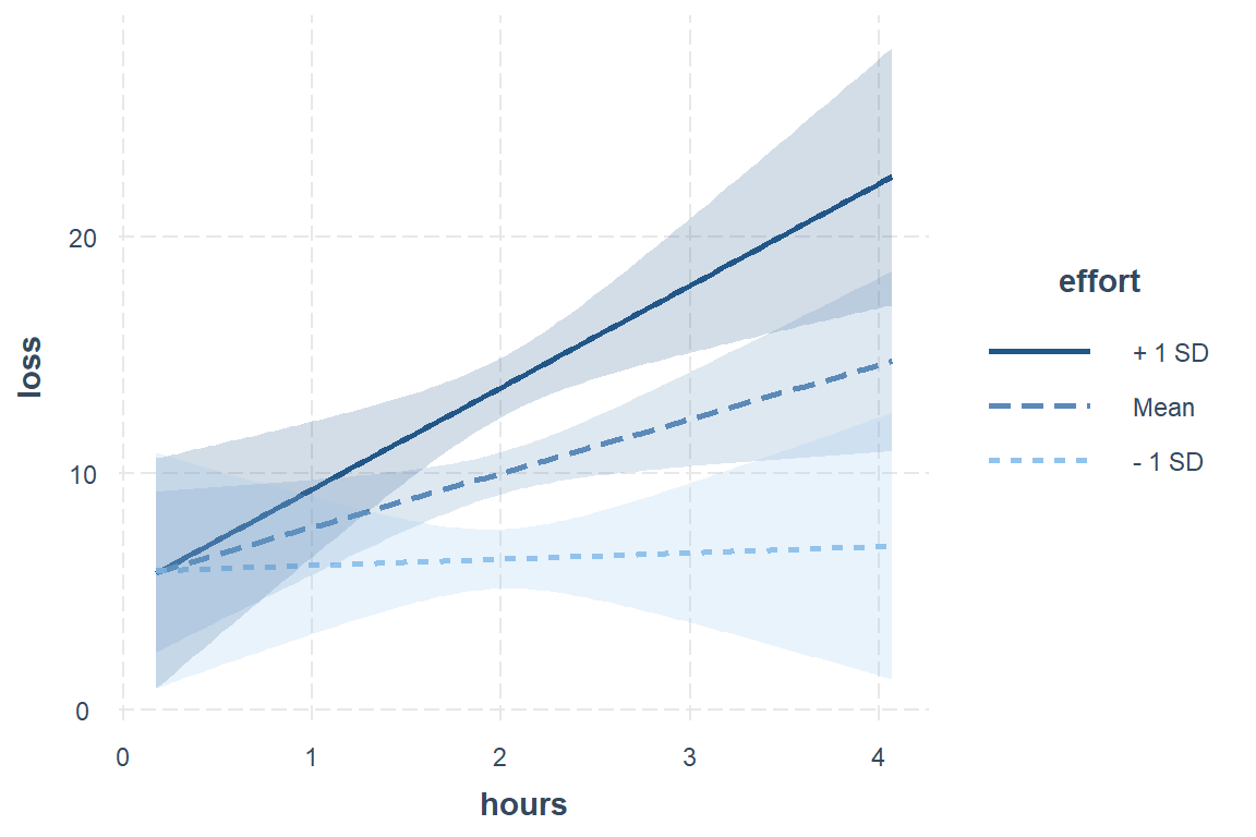
Since these packages are built on ggplot2 you can customise them further to make them ‘better’ for publication.
fit_lm_loss_hr_eff %>%
  interactions::interact_plot(pred = hours,
                              modx = effort,
                              interval = TRUE,
                              int.type = "confidence",
                              legend.main = "Effort:") +
  labs(x = "Hours Spent Exercising",
       y = "Weight Loss, pounds") +
  theme_bw() +
  theme(legend.position = c(0, 1),
        legend.justification = c(-0.1, 1.1),
        legend.background = element_rect(color = "black"),
        legend.key.width = unit(1.5, "cm"))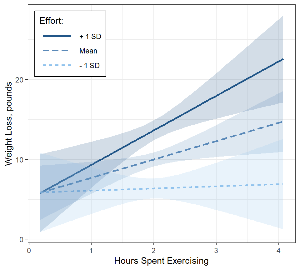
fit_lm_loss_hr_eff %>%
  interactions::interact_plot(pred = hours,
                              modx = effort,
                              modx.values = c(15, 24, 35, 45),
                              interval = TRUE,
                              int.type = "confidence",
                              legend.main = "Effort:") +
  labs(x = "Hours Spent Exercising",
       y = "Weight Loss, pounds") +
  geom_hline(yintercept = 0) +
  theme_bw() +
  theme(legend.position = c(0, 1),
        legend.justification = c(-0.1, 1.1),
        legend.background = element_rect(color = "black"),
        legend.key.width = unit(1.5, "cm"))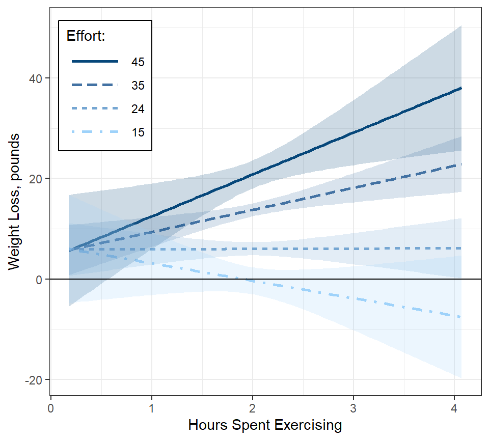
Interpretation: When little time is spent on the program, participants lost just over 5 pounds, irrespective of effort. More time spent on the programs only translated to additional weight lost if their effort was high.
6.5.5 Predict and Pairwise Tests
By default, we get a prediction for the mean hours (2) and the mean effort (29.7).
fit_lm_loss_hr_eff %>%
  emmeans::emmeans(~ hours*effort)
hours effort emmean SE df lower.CL upper.CL
2 29.7 10 0.452 896 9.12 10.9
Confidence level used: 0.95 We can customize which hours and effort for which we want to get predictions for.
fit_lm_loss_hr_eff %>%
  emmeans::emmeans(~ hours*effort,
                   at = list(hours = 1:4,
                             effort = c(20, 30, 40)))
hours effort emmean SE df lower.CL upper.CL
1 20 4.684 2.253 896 0.262 9.11
2 20 3.176 0.962 896 1.287 5.06
3 20 1.667 2.284 896 -2.815 6.15
4 20 0.158 4.236 896 -8.156 8.47
1 30 7.815 1.024 896 5.805 9.82
2 30 10.240 0.453 896 9.351 11.13
3 30 12.665 1.019 896 10.665 14.66
4 30 15.089 1.883 896 11.394 18.78
1 40 10.946 2.357 896 6.319 15.57
2 40 17.304 1.016 896 15.311 19.30
3 40 23.662 2.341 896 19.068 28.26
4 40 30.020 4.348 896 21.488 38.55
Confidence level used: 0.95 By adding the word pairwise we also get pairwise t-tests! Tukey’s HSD adjustment for multiple compairisons is done by default.
fit_lm_loss_hr_eff %>%
  emmeans::emmeans(pairwise ~ hours*effort,
                   at = list(hours = 2:3,
                             effort = c(25, 35)))
$emmeans
hours effort emmean SE df lower.CL upper.CL
2 25 6.71 0.610 896 5.51 7.91
3 25 7.17 1.431 896 4.36 9.98
2 35 13.77 0.652 896 12.49 15.05
3 35 18.16 1.477 896 15.26 21.06
Confidence level used: 0.95
$contrasts
contrast estimate SE df t.ratio p.value
2 25 - 3 25 -0.458 1.28 896 -0.357 0.9845
2 25 - 2 35 -7.064 0.88 896 -8.031 <.0001
2 25 - 3 35 -11.456 1.59 896 -7.186 <.0001
3 25 - 2 35 -6.606 1.57 896 -4.212 0.0002
3 25 - 3 35 -10.998 2.08 896 -5.297 <.0001
2 35 - 3 35 -4.391 1.34 896 -3.288 0.0058
P value adjustment: tukey method for comparing a family of 4 estimates By changing the astrics (*) to a vertical bar (|) we get compairisons between different hours WITHIN each effort level.
fit_lm_loss_hr_eff %>%
  emmeans::emmeans(pairwise ~ hours|effort,
                   at = list(hours = c(1, 4),
                             effort = c(20, 30, 40)))
$emmeans
effort = 20:
hours emmean SE df lower.CL upper.CL
1 4.684 2.25 896 0.262 9.11
4 0.158 4.24 896 -8.156 8.47
effort = 30:
hours emmean SE df lower.CL upper.CL
1 7.815 1.02 896 5.805 9.82
4 15.089 1.88 896 11.394 18.78
effort = 40:
hours emmean SE df lower.CL upper.CL
1 10.946 2.36 896 6.319 15.57
4 30.020 4.35 896 21.488 38.55
Confidence level used: 0.95
$contrasts
effort = 20:
contrast estimate SE df t.ratio p.value
1 - 4 4.53 6.16 896 0.734 0.4629
effort = 30:
contrast estimate SE df t.ratio p.value
1 - 4 -7.27 2.75 896 -2.649 0.0082
effort = 40:
contrast estimate SE df t.ratio p.value
1 - 4 -19.07 6.35 896 -3.002 0.00286.5.6 Simple Slopes Analysis
By default, we only get the overall slope for time spent for the mean effort (29.7) and plus-or-minus one standard deviation (24.51 & 34.80).
fit_lm_loss_hr_eff %>%
  interactions::sim_slopes(pred = hours,
                           modx = effort)
JOHNSON-NEYMAN INTERVAL
When effort is OUTSIDE the interval [-64.73, 28.55], the slope of hours is
p < .05.
Note: The range of observed values of effort is [12.95, 44.08]
SIMPLE SLOPES ANALYSIS
Slope of hours when effort = 24.51646 (- 1 SD):
Est. S.E. t val. p
------ ------ -------- ------
0.27 1.35 0.20 0.84
Slope of hours when effort = 29.65922 (Mean):
Est. S.E. t val. p
------ ------ -------- ------
2.29 0.92 2.50 0.01
Slope of hours when effort = 34.80198 (+ 1 SD):
Est. S.E. t val. p
------ ------ -------- ------
4.31 1.31 3.30 0.00You may specify other specific values.
fit_lm_loss_hr_eff %>%
  interactions::sim_slopes(pred = hours,
                           modx = effort,
                           modx.values = c(15, 25, 23, 45))
JOHNSON-NEYMAN INTERVAL
When effort is OUTSIDE the interval [-64.73, 28.55], the slope of hours is
p < .05.
Note: The range of observed values of effort is [12.95, 44.08]
SIMPLE SLOPES ANALYSIS
Slope of hours when effort = 15.00:
Est. S.E. t val. p
------- ------ -------- ------
-3.48 2.92 -1.19 0.23
Slope of hours when effort = 25.00:
Est. S.E. t val. p
------ ------ -------- ------
0.46 1.28 0.36 0.72
Slope of hours when effort = 23.00:
Est. S.E. t val. p
------- ------ -------- ------
-0.33 1.57 -0.21 0.83
Slope of hours when effort = 45.00:
Est. S.E. t val. p
------ ------ -------- ------
8.32 2.99 2.78 0.016.6 Continuous by Categorical
6.6.1 Fit MLR Model
Question: Did weight loss depend on gender?
fit_lm_loss_gen <- lm(loss ~ gender,
data = data_clean)summary(fit_lm_loss_gen)
Call:
lm(formula = loss ~ gender, data = data_clean)

Residuals:
    Min      1Q  Median      3Q     Max
-27.067 -11.788  -2.156   9.977  44.222

Coefficients:
             Estimate Std. Error t value Pr(>|t|)
(Intercept)   10.1129     0.6650  15.206   <2e-16 ***
genderFemale  -0.1842     0.9405  -0.196    0.845
---
Signif. codes:  0 '***' 0.001 '**' 0.01 '*' 0.05 '.' 0.1 ' ' 1

Residual standard error: 14.11 on 898 degrees of freedom
Multiple R-squared:  4.271e-05, Adjusted R-squared:  -0.001071
F-statistic: 0.03835 on 1 and 898 DF, p-value: 0.8448Answer:The main effect of gender is not significant.
Question: Does gender moderate the effect of spending addition time on the program? (ignoring the role of effort and program type for the time being)
fit_lm_loss_hrs_gen <- lm(loss ~ hours*gender,
data = data_clean)summary(fit_lm_loss_hrs_gen)
Call:
lm(formula = loss ~ hours * gender, data = data_clean)

Residuals:
    Min      1Q  Median      3Q     Max
-27.118 -11.350  -1.963  10.001  42.376

Coefficients:
                   Estimate Std. Error t value Pr(>|t|)
(Intercept)           6.906      2.805   2.462    0.014 *
hours                 1.591      1.352   1.177    0.240
genderFemale         -3.571      3.915  -0.912    0.362
hours:genderFemale    1.724      1.898   0.908    0.364
---
Signif. codes:  0 '***' 0.001 '**' 0.01 '*' 0.05 '.' 0.1 ' ' 1

Residual standard error: 14.06 on 896 degrees of freedom
Multiple R-squared:  0.008433,  Adjusted R-squared:  0.005113
F-statistic:  2.54 on 3 and 896 DF,  p-value: 0.05523
Answer: No, gender does not interact with time spent.
Question: Is the effect of time spend moderated by type of program?
fit_lm_loss_prog <- lm(loss ~ prog,
data = data_clean)summary(fit_lm_loss_prog)
Call:
lm(formula = loss ~ prog, data = data_clean)

Residuals:
     Min       1Q   Median       3Q      Max
-22.4700  -4.6636  -0.0762   4.1810  28.3304

Coefficients:
            Estimate Std. Error t value Pr(>|t|)
(Intercept)   8.0304     0.4110   19.54   <2e-16 ***
progSwim     17.7897     0.5813   30.61   <2e-16 ***
progRead    -11.8182     0.5813  -20.33   <2e-16 ***
---
Signif. codes:  0 '***' 0.001 '**' 0.01 '*' 0.05 '.' 0.1 ' ' 1

Residual standard error: 7.119 on 897 degrees of freedom
Multiple R-squared:  0.7457,    Adjusted R-squared:  0.7451
F-statistic:  1315 on 2 and 897 DF,  p-value: < 2.2e-16
fit_lm_loss_hrs_prog <- lm(loss ~ hours*prog,
data = data_clean)summary(fit_lm_loss_hrs_prog)
Call:
lm(formula = loss ~ hours * prog, data = data_clean)

Residuals:
    Min      1Q  Median      3Q     Max
-24.977  -4.146  -0.213   3.992  25.067

Coefficients:
               Estimate Std. Error t value Pr(>|t|)
(Intercept)     -6.7807     1.6438  -4.125 4.06e-05 ***
hours            7.4527     0.8053   9.255  < 2e-16 ***
progSwim        18.9296     2.2877   8.275 4.66e-16 ***
progRead         8.9970     2.2160   4.060 5.34e-05 ***
hours:progSwim  -0.5787     1.1193  -0.517    0.605
hours:progRead -10.4089     1.0723  -9.708  < 2e-16 ***
---
Signif. codes:  0 '***' 0.001 '**' 0.01 '*' 0.05 '.' 0.1 ' ' 1

Residual standard error: 6.502 on 894 degrees of freedom
Multiple R-squared:  0.7885,    Adjusted R-squared:  0.7874
F-statistic: 666.8 on 5 and 894 DF, p-value: < 2.2e-16anova(fit_lm_loss_hrs_prog)# A tibble: 4 x 5
Df `Sum Sq` `Mean Sq` `F value` `Pr(>F)`
<int> <dbl> <dbl> <dbl> <dbl>
1 1 1341. 1341. 31.7 2.39e- 8
2 2 134281. 67140. 1588. 5.60e-295
3 2 5319. 2660. 62.9 2.75e- 26
4 894 37795. 42.3 NA NA Answer: Yes! The type of program does moderate the effect of time spent on weight loss, F(2, 894) = 62.91, p < .001.
6.6.2 Table Comparing Models
Sometimes its nice to have a table of the parameter estimates of competing models.
texreg::screenreg(list(fit_lm_loss_hr,
                       fit_lm_loss_gen,
                       fit_lm_loss_prog,
                       fit_lm_loss_hrs_gen,
                       fit_lm_loss_hrs_prog),
                  custom.model.names = c("Hrs",
                                         "Gender",
                                         "Program",
                                         "Hrs + Gender",
                                         "Hrs + Program"))
==================================================================================
                    Hrs        Gender      Program     Hrs + Gender  Hrs + Program
----------------------------------------------------------------------------------
(Intercept)           5.08 **   10.11 ***    8.03 ***    6.91 *       -6.78 ***
                     (1.96)     (0.67)      (0.41)      (2.81)        (1.64)
hours                 2.47 **                            1.59          7.45 ***
                     (0.95)                             (1.35)        (0.81)
genderFemale                    -0.18                   -3.57
                                (0.94)                  (3.91)
progSwim                                    17.79 ***                 18.93 ***
                                            (0.58)                    (2.29)
progRead                                   -11.82 ***                  9.00 ***
                                            (0.58)                    (2.22)
hours:genderFemale                                       1.72
                                                        (1.90)
hours:progSwim                                                        -0.58
                                                                      (1.12)
hours:progRead                                                       -10.41 ***
                                                                      (1.07)
----------------------------------------------------------------------------------
R^2                   0.01       0.00        0.75        0.01          0.79
Adj. R^2              0.01      -0.00        0.75        0.01          0.79
Num. obs.           900        900         900         900           900
==================================================================================
*** p < 0.001; ** p < 0.01; * p < 0.05
6.6.3 Check Assumptions
par(mfrow = c(2, 2))
plot(fit_lm_loss_hrs_prog)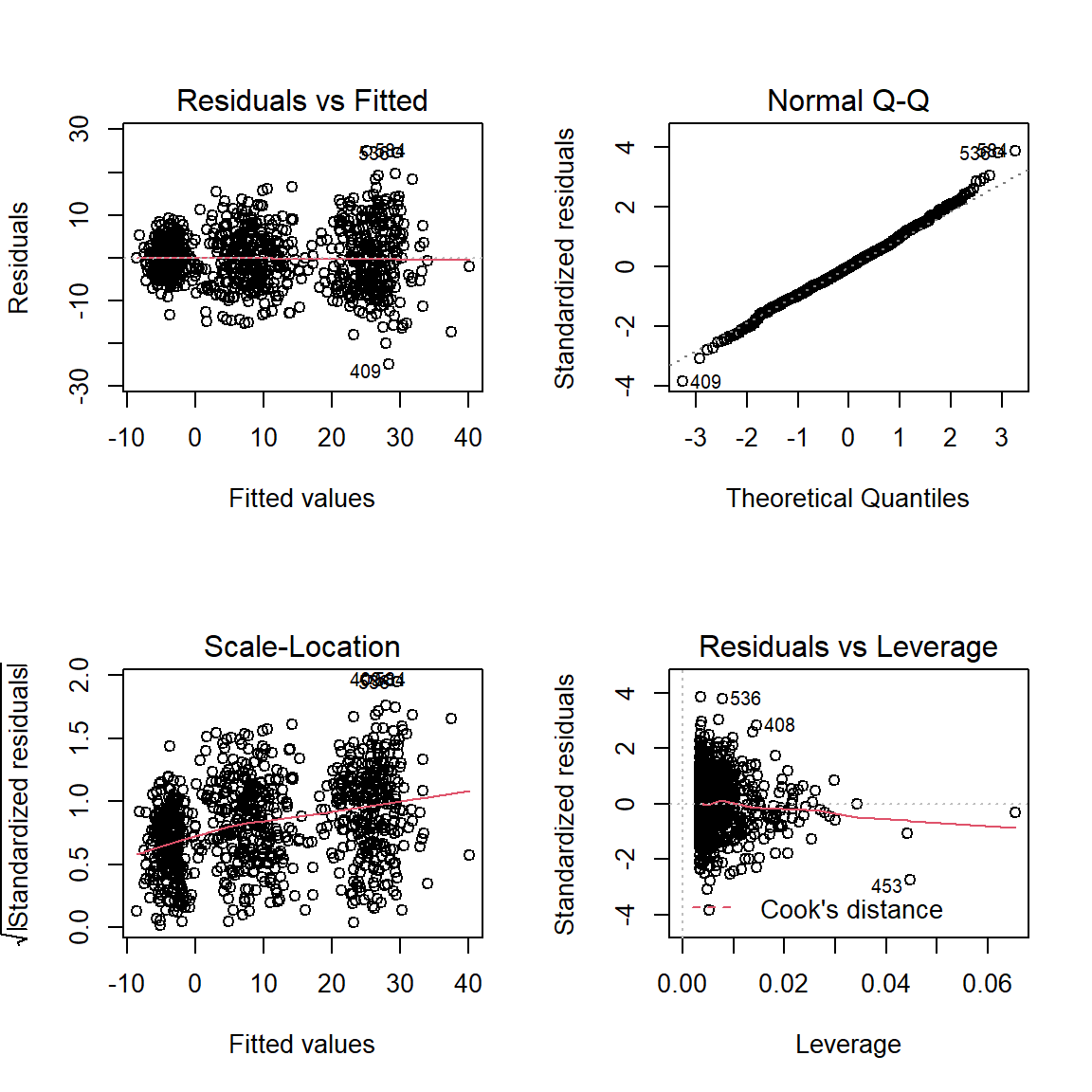
par(mfrow = c(1, 1))6.6.4 Plot Estimated Marginal Means
fit_lm_loss_hrs_prog %>%
  interactions::interact_plot(pred = hours,
                              modx = prog,
                              interval = TRUE,
                              int.type = "confidence",
                              legend.main = "Program:") +
  theme_bw() +
  theme(legend.background = element_rect(color = "black"),
        legend.position = c(0, 1),
        legend.justification = c(-0.1, 1.1),
        legend.key.width = unit(2, "cm")) +
  labs(x = "Time Spend on Program, hours",
       y = "Weight Loss, pounds",
       caption = "Note. Bands represent 95% confidence intervals") +
  geom_hline(yintercept = 0)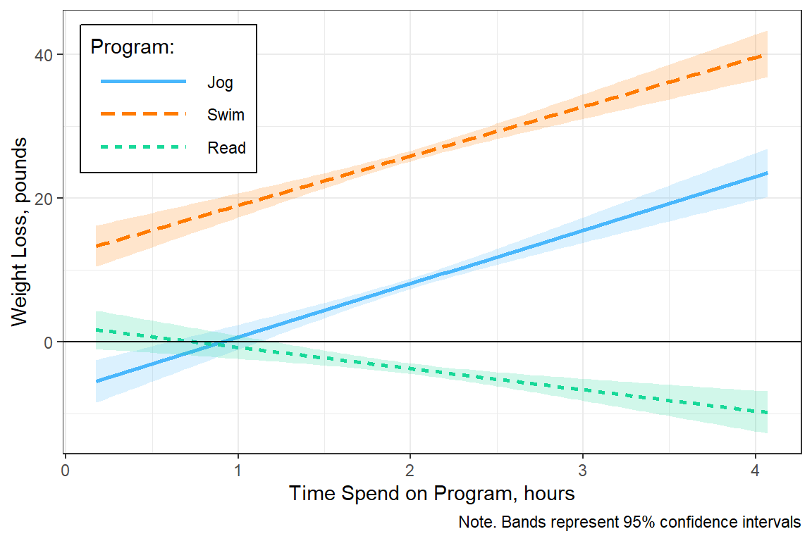
6.6.5 Predict and Pairwise Tests
fit_lm_loss_hrs_prog %>%
  emmeans::emmeans(~hours)
hours emmean SE df lower.CL upper.CL
2 10.1 0.217 894 9.69 10.5
Results are averaged over the levels of: prog
Confidence level used: 0.95 fit_lm_loss_hrs_prog %>%
emmeans::emmeans(~ prog) prog emmean SE df lower.CL upper.CL
Jog 8.14 0.376 894 7.41 8.88
Swim 25.91 0.376 894 25.18 26.65
Read -3.70 0.376 894 -4.44 -2.97
Confidence level used: 0.95 fit_lm_loss_hrs_prog %>%
emmeans::emmeans(~ hours|prog)prog = Jog:
hours emmean SE df lower.CL upper.CL
2 8.14 0.376 894 7.41 8.88
prog = Swim:
hours emmean SE df lower.CL upper.CL
2 25.91 0.376 894 25.18 26.65
prog = Read:
hours emmean SE df lower.CL upper.CL
2 -3.70 0.376 894 -4.44 -2.97
Confidence level used: 0.95 fit_lm_loss_hrs_prog %>%
emmeans::emmeans(~ hours|prog,
at = list(hours = 1:4))prog = Jog:
hours emmean SE df lower.CL upper.CL
1 0.672 0.879 894 -1.05 2.398
2 8.125 0.376 894 7.39 8.862
3 15.578 0.898 894 13.82 17.340
4 23.030 1.664 894 19.77 26.296
prog = Swim:
hours emmean SE df lower.CL upper.CL
1 19.023 0.855 894 17.34 20.702
2 25.897 0.375 894 25.16 26.634
3 32.771 0.871 894 31.06 34.481
4 39.645 1.608 894 36.49 42.801
prog = Read:
hours emmean SE df lower.CL upper.CL
1 -0.740 0.821 894 -2.35 0.871
2 -3.696 0.376 894 -4.43 -2.958
3 -6.652 0.782 894 -8.19 -5.117
4 -9.608 1.444 894 -12.44 -6.775
Confidence level used: 0.95 6.6.6 Simple Slopes Analysis
fit_lm_loss_hrs_prog %>%
  interactions::sim_slopes(pred = hours,
                           modx = prog)
SIMPLE SLOPES ANALYSIS
Slope of hours when prog = Read:
Est. S.E. t val. p
------- ------ -------- ------
-2.96 0.71 -4.18 0.00
Slope of hours when prog = Swim:
Est. S.E. t val. p
------ ------ -------- ------
6.87 0.78 8.84 0.00
Slope of hours when prog = Jog:
Est. S.E. t val. p
------ ------ -------- ------
7.45 0.81 9.25 0.00Interpretation: Participants in the jogging program (M = 7.45 lb/hr, SE = 0.81) and the swimming program (M = 6.87 lb/hr, SE = 0.78), loose about the same amount of weight for each additional hour spent exercising, p = .863, conversely, each additional hour reading is associated with more weight gained (M = -2.96 lb/hr, SE = 0.71).
6.7 Categorical by Categorical
6.7.1 Fit MLR Model
Question: Do both genders have the same success in all the programs?
fit_lm_loss_prog <- lm(loss ~ prog,
                       data = data_clean)

fit_lm_loss_prog_gen <- lm(loss ~ prog*gender,
data = data_clean)summary(fit_lm_loss_prog_gen)
Call:
lm(formula = loss ~ prog * gender, data = data_clean)

Residuals:
     Min       1Q   Median       3Q      Max
-19.1723  -4.1894  -0.0994   3.7506  27.6939

Coefficients:
                      Estimate Std. Error t value Pr(>|t|)
(Intercept)            11.7720     0.5322  22.118  < 2e-16 ***
progSwim               10.7504     0.7527  14.282  < 2e-16 ***
progRead              -15.7276     0.7527 -20.895  < 2e-16 ***
genderFemale           -7.4833     0.7527  -9.942  < 2e-16 ***
progSwim:genderFemale  14.0787     1.0645  13.226  < 2e-16 ***
progRead:genderFemale   7.8188     1.0645   7.345 4.63e-13 ***
---
Signif. codes:  0 '***' 0.001 '**' 0.01 '*' 0.05 '.' 0.1 ' ' 1

Residual standard error: 6.519 on 894 degrees of freedom
Multiple R-squared:  0.7875,    Adjusted R-squared:  0.7863
F-statistic: 662.5 on 5 and 894 DF, p-value: < 2.2e-16anova(fit_lm_loss_prog_gen)# A tibble: 4 x 5
Df `Sum Sq` `Mean Sq` `F value` `Pr(>F)`
<int> <dbl> <dbl> <dbl> <dbl>
1 2 133277. 66639. 1568. 4.49e-293
2 1 7.63 7.63 0.180 6.72e- 1
3 2 7463. 3732. 87.8 1.51e- 35
4 894 37988. 42.5 NA NA Answer: At least one of the programs results in more weight lost for one of the genders.
6.7.2 Table of Parameter Estimates
texreg::screenreg(list(fit_lm_loss_gen,
                       fit_lm_loss_prog,
                       fit_lm_loss_prog_gen),
                  custom.model.names = c("Gender",
                                         "Program",
                                         "Interacting"))
==========================================================
                       Gender      Program     Interacting
----------------------------------------------------------
(Intercept)             10.11 ***    8.03 ***   11.77 ***
                        (0.67)      (0.41)      (0.53)
genderFemale            -0.18                   -7.48 ***
                        (0.94)                  (0.75)
progSwim                            17.79 ***   10.75 ***
                                    (0.58)      (0.75)
progRead                           -11.82 ***  -15.73 ***
                                    (0.58)      (0.75)
progSwim:genderFemale                           14.08 ***
                                                (1.06)
progRead:genderFemale                            7.82 ***
                                                (1.06)
----------------------------------------------------------
R^2                      0.00        0.75        0.79
Adj. R^2                -0.00        0.75        0.79
Num. obs.              900         900         900
==========================================================
*** p < 0.001; ** p < 0.01; * p < 0.05
6.7.3 Check Assumptions
par(mfrow = c(2, 2))
plot(fit_lm_loss_prog_gen)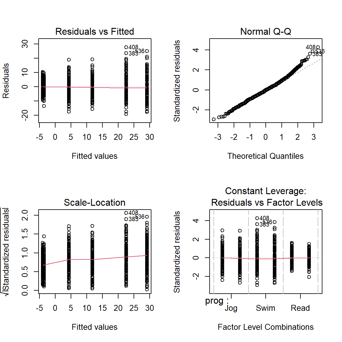
par(mfrow = c(1, 1))6.7.4 Plot Estimated Marginal Means
fit_lm_loss_prog_gen %>%
  interactions::cat_plot(pred = prog,
                         modx = gender)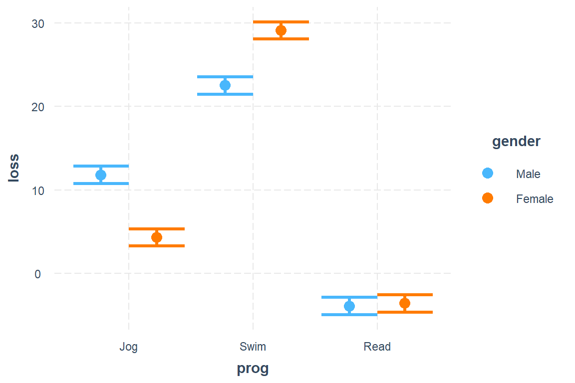
fit_lm_loss_prog_gen %>%
  interactions::cat_plot(pred = prog,
                         modx = gender,
                         geom = "line",
                         dodge.width = .2,
                         errorbar.width = .25,
                         point.shape = TRUE,
                         # vary.lty = TRUE,
                         colors = c("gray10", "gray50"),
                         legend.main = "Gender:") +
  theme_bw() +
  theme(legend.background = element_rect(color = "black"),
        legend.position = c(0, 1),
        legend.justification = c(-0.1, 1.1),
        legend.key.width = unit(2, "cm")) +
  labs(x = "Program",
       y = "Weight Loss, pounds",
       caption = "Note. Error Bars represent 95% confidence intervals") +
  geom_hline(yintercept = 0) +
  scale_shape_manual("Gender:", values = c(15, 16))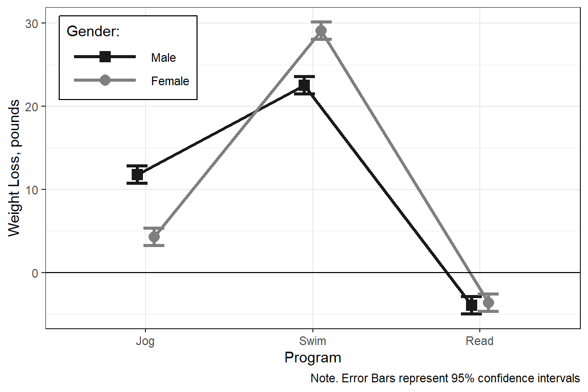
6.7.5 Predict and Pairwise Tests
Question: Which gender or program looses the most and least weight?
fit_lm_loss_prog_gen %>%
  emmeans::emmeans(pairwise ~ prog | gender)
$emmeans
gender = Male:
prog emmean SE df lower.CL upper.CL
Jog 11.77 0.532 894 10.73 12.82
Swim 22.52 0.532 894 21.48 23.57
Read -3.96 0.532 894 -5.00 -2.91
gender = Female:
prog emmean SE df lower.CL upper.CL
Jog 4.29 0.532 894 3.24 5.33
Swim 29.12 0.532 894 28.07 30.16
Read -3.62 0.532 894 -4.66 -2.58
Confidence level used: 0.95
$contrasts
gender = Male:
contrast estimate SE df t.ratio p.value
Jog - Swim -10.75 0.753 894 -14.282 <.0001
Jog - Read 15.73 0.753 894 20.895 <.0001
Swim - Read 26.48 0.753 894 35.177 <.0001
gender = Female:
contrast estimate SE df t.ratio p.value
Jog - Swim -24.83 0.753 894 -32.986 <.0001
Jog - Read 7.91 0.753 894 10.507 <.0001
Swim - Read 32.74 0.753 894 43.494 <.0001
P value adjustment: tukey method for comparing a family of 3 estimates Answer: For each gender, the swimming program resultsed in the most weight lost, followed by the jogging program, where as the the reading program paticipants gained weight.
fit_lm_loss_prog_gen %>%
  emmeans::emmeans(pairwise ~ gender | prog)
$emmeans
prog = Jog:
gender emmean SE df lower.CL upper.CL
Male 11.77 0.532 894 10.73 12.82
Female 4.29 0.532 894 3.24 5.33
prog = Swim:
gender emmean SE df lower.CL upper.CL
Male 22.52 0.532 894 21.48 23.57
Female 29.12 0.532 894 28.07 30.16
prog = Read:
gender emmean SE df lower.CL upper.CL
Male -3.96 0.532 894 -5.00 -2.91
Female -3.62 0.532 894 -4.66 -2.58
Confidence level used: 0.95
$contrasts
prog = Jog:
contrast estimate SE df t.ratio p.value
Male - Female 7.483 0.753 894 9.942 <.0001
prog = Swim:
contrast estimate SE df t.ratio p.value
Male - Female -6.595 0.753 894 -8.762 <.0001
prog = Read:
contrast estimate SE df t.ratio p.value
Male - Female -0.335 0.753 894 -0.446 0.6559Answer: In the swimming program females lost more weight than males, but the reverse trend was observed in the jogging group. In the reading group there was no gender gap in weight lost.
6.7.6 Simple Slopes Analysis
Not appropriate for categorical-only interactions
6.8 Three-way Interaction
6.8.1 Fit MLR Models
fit_lm_loss_3way_a <- lm(loss ~ prog*gender*effort,
data = data_clean)summary(fit_lm_loss_3way_a)
Call:
lm(formula = loss ~ prog * gender * effort, data = data_clean)

Residuals:
    Min      1Q  Median      3Q     Max
-19.455  -3.266  -0.009   3.128  15.941

Coefficients:
                              Estimate Std. Error t value Pr(>|t|)
(Intercept)                  -13.99416    2.44383  -5.726 1.40e-08 ***
progSwim                       2.14594    3.43352   0.625  0.53213
progRead                       7.85129    3.41229   2.301  0.02163 *
genderFemale                  -0.31768    3.53356  -0.090  0.92838
effort                         0.85225    0.07968  10.696  < 2e-16 ***
progSwim:genderFemale          5.81629    4.89795   1.187  0.23535
progRead:genderFemale          1.99989    4.85732   0.412  0.68064
progSwim:effort                0.30249    0.11280   2.682  0.00746 **
progRead:effort               -0.77742    0.11308  -6.875 1.17e-11 ***
genderFemale:effort           -0.22963    0.11601  -1.979  0.04807 *
progSwim:genderFemale:effort   0.27596    0.16174   1.706  0.08832 .
progRead:genderFemale:effort   0.18347    0.16131   1.137  0.25570
---
Signif. codes:  0 '***' 0.001 '**' 0.01 '*' 0.05 '.' 0.1 ' ' 1

Residual standard error: 5.041 on 888 degrees of freedom
Multiple R-squared:  0.8738,    Adjusted R-squared:  0.8722
F-statistic: 558.8 on 11 and 888 DF, p-value: < 2.2e-16anova(fit_lm_loss_3way_a)# A tibble: 8 x 5
Df `Sum Sq` `Mean Sq` `F value` `Pr(>F)`
<int> <dbl> <dbl> <dbl> <dbl>
1 2 133277. 66639. 2623. 0
2 1 7.63 7.63 0.300 5.84e- 1
3 1 10220. 10220. 402. 4.37e-74
4 2 7361. 3681. 145. 3.57e-55
5 2 5200. 2600. 102. 1.03e-40
6 1 31.9 31.9 1.26 2.63e- 1
7 2 76.3 38.1 1.50 2.24e- 1
8 888 22563. 25.4 NA NA fit_lm_loss_3way_b <- lm(loss ~ prog*gender*hours,
data = data_clean)summary(fit_lm_loss_3way_b)
Call:
lm(formula = loss ~ prog * gender * hours, data = data_clean)

Residuals:
     Min       1Q   Median       3Q      Max
-22.5750  -3.6364  -0.2174   3.7454  22.6508

Coefficients:
                            Estimate Std. Error t value Pr(>|t|)
(Intercept)                   2.9697     2.0709   1.434 0.151920
progSwim                      1.6405     2.8765   0.570 0.568597
progRead                      0.8296     2.8621   0.290 0.771979
genderFemale                -17.8974     2.9467  -6.074 1.85e-09 ***
hours                         4.3646     0.9995   4.367 1.41e-05 ***
progSwim:genderFemale        33.6854     4.0969   8.222 7.06e-16 ***
progRead:genderFemale        14.9821     3.9766   3.768 0.000176 ***
progSwim:hours                4.6917     1.4001   3.351 0.000839 ***
progRead:hours               -8.1430     1.3682  -5.952 3.82e-09 ***
genderFemale:hours            5.4500     1.4445   3.773 0.000172 ***
progSwim:genderFemale:hours -10.1461     2.0052  -5.060 5.10e-07 ***
progRead:genderFemale:hours  -3.9129     1.9242  -2.033 0.042302 *
---
Signif. codes:  0 '***' 0.001 '**' 0.01 '*' 0.05 '.' 0.1 ' ' 1

Residual standard error: 5.814 on 888 degrees of freedom
Multiple R-squared:  0.832, Adjusted R-squared:   0.83
F-statistic: 399.9 on 11 and 888 DF, p-value: < 2.2e-16anova(fit_lm_loss_3way_b)# A tibble: 8 x 5
Df `Sum Sq` `Mean Sq` `F value` `Pr(>F)`
<int> <dbl> <dbl> <dbl> <dbl>
1 2 133277. 66639. 1971. 0
2 1 7.63 7.63 0.226 6.35e- 1
3 1 2339. 2339. 69.2 3.35e-16
4 2 7202. 3601. 107. 3.46e-42
5 2 4973. 2486. 73.5 2.79e-30
6 1 27.0 27.0 0.798 3.72e- 1
7 2 889. 445. 13.2 2.35e- 6
8 888 30022. 33.8 NA NA 6.8.2 Table of Parameter Estimates
We can ask the table to show confidence intervals (95% by default) instead of standard errors.
texreg::screenreg(list(fit_lm_loss_3way_b),
                  single.row = TRUE,
                  ci.force = TRUE)
======================================================
                             Model 1
------------------------------------------------------
(Intercept)                    2.97 [ -1.09;   7.03]
progSwim                       1.64 [ -4.00;   7.28]
progRead                       0.83 [ -4.78;   6.44]
genderFemale                 -17.90 [-23.67; -12.12] *
hours                          4.36 [  2.41;   6.32] *
progSwim:genderFemale         33.69 [ 25.66;  41.72] *
progRead:genderFemale         14.98 [  7.19;  22.78] *
progSwim:hours                 4.69 [  1.95;   7.44] *
progRead:hours                -8.14 [-10.82;  -5.46] *
genderFemale:hours             5.45 [  2.62;   8.28] *
progSwim:genderFemale:hours  -10.15 [-14.08;  -6.22] *
progRead:genderFemale:hours   -3.91 [ -7.68;  -0.14] *
------------------------------------------------------
R^2                            0.83
Adj. R^2                       0.83
Num. obs.                    900
======================================================
* 0 outside the confidence interval.
6.8.3 Check Assumptions
par(mfrow = c(2, 2))
plot(fit_lm_loss_3way_b)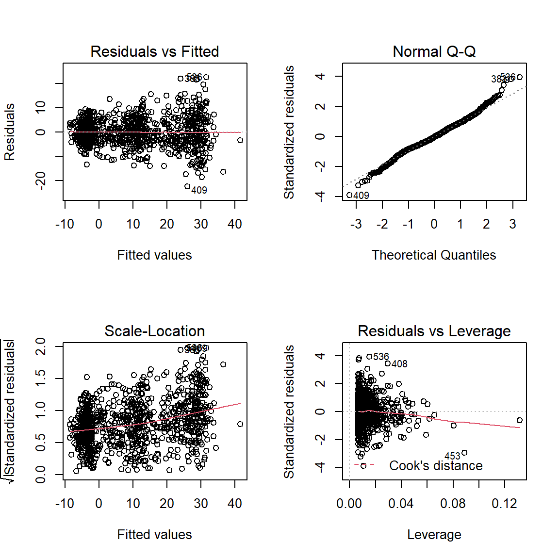
par(mfrow = c(1, 1))6.8.4 Plot Estimated Marginal Means
fit_lm_loss_3way_b %>%
  interactions::interact_plot(pred = hours,            # x-axis
                              modx = prog,             # separate lines
                              mod2 = gender,           # separate panels
                              interval = TRUE,         # add bands
                              int.type = "confidence",
                              legend.main = "Program:") +
  theme_bw() +
  theme(legend.background = element_rect(color = "black"),
        legend.position = c(0, 1),
        legend.justification = c(-0.1, 1.1),
        legend.key.width = unit(1.5, "cm")) +
  labs(x = "Time Spend on Program, hours",
       y = "Weight Loss, pounds",
       caption = "Note. Bands represent 95% confidence intervals") +
  geom_hline(yintercept = 0)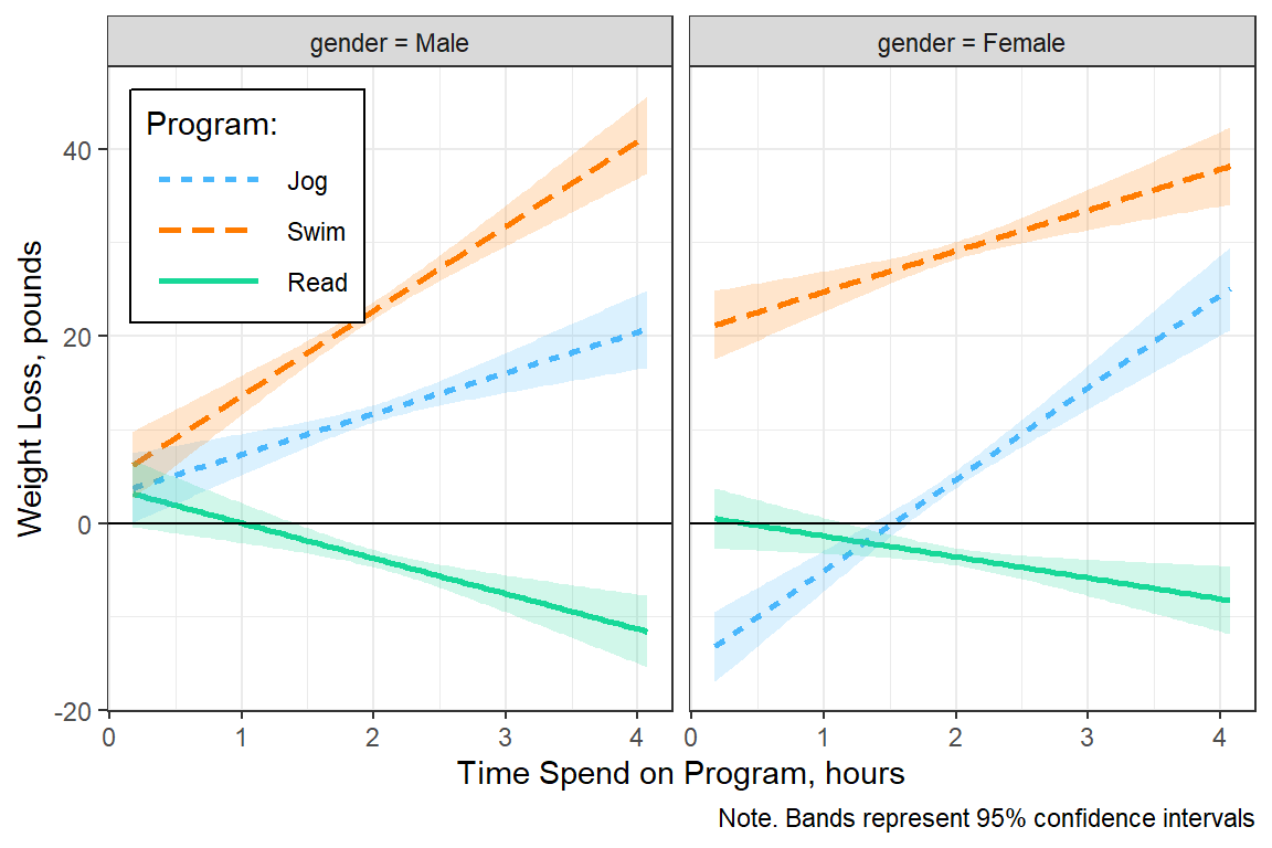
fit_lm_loss_3way_b %>%
  interactions::interact_plot(pred = hours,            # x-axis
                              modx = gender,           # separate lines
                              mod2 = prog,             # separate panels
                              interval = TRUE,         # add bands
                              int.type = "confidence",
                              legend.main = "Gender:") +
  theme_bw() +
  theme(legend.background = element_rect(color = "black"),
        legend.position = c(0, 1),
        legend.justification = c(-0.1, 1.1),
        legend.key.width = unit(1.5, "cm")) +
  labs(x = "Time Spend on Program, hours",
       y = "Weight Loss, pounds",
       caption = "Note. Bands represent 95% confidence intervals") +
  geom_hline(yintercept = 0)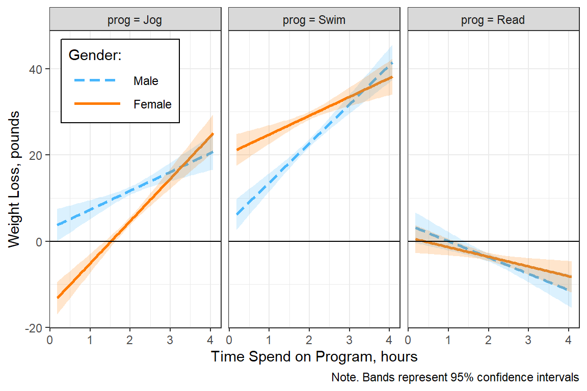
6.8.5 Simple Slopes Analysis
By default, we only get the overall slope for time spent for the mean effort (29.7) and plus-or-minus one standard deviation (24.51 & 34.80).
fit_lm_loss_3way_b %>%
  interactions::sim_slopes(pred = hours,
                           modx = prog,
                           mod2 = gender)
###################### While gender (2nd moderator) = Male #####################
SIMPLE SLOPES ANALYSIS
Slope of hours when prog = Jog:
Est. S.E. t val. p
------ ------ -------- ------
4.36 1.00 4.37 0.00
Slope of hours when prog = Swim:
Est. S.E. t val. p
------ ------ -------- ------
9.06 0.98 9.24 0.00
Slope of hours when prog = Read:
Est. S.E. t val. p
------- ------ -------- ------
-3.78 0.93 -4.04 0.00
##################### While gender (2nd moderator) = Female ####################
SIMPLE SLOPES ANALYSIS
Slope of hours when prog = Jog:
Est. S.E. t val. p
------ ------ -------- ------
9.81 1.04 9.41 0.00
Slope of hours when prog = Swim:
Est. S.E. t val. p
------ ------ -------- ------
4.36 0.99 4.42 0.00
Slope of hours when prog = Read:
Est. S.E. t val. p
------- ------ -------- ------
-2.24 0.86 -2.60 0.01