7 Interactions Example
library(tidyverse)
library(emmeans)
library(furniture)
library(stargazer)
library(psych)
library(texreg)
library(interactions)
library(rgl)
Regression Analysis and Linear Models: concepts, applicaitons, and implementation - By Richard B. Darlington & Andrew F. Hayes
Chapter 3: Partial Relationships and the Multiple Linear Regressio Model
7.1 The Data
Data from Table 3.1
df <- data.frame(id = 1:10,
                 exercise = c( 0,  0,  0,  2,  2,  2,  2,  4,  4,  4),
                 food     = c( 2,  4,  6,  2,  4,  6,  8,  4,  6,  8),
                 metabo   = c(15, 14, 19, 15, 21, 23, 21, 22, 24, 26),
                 loss     = c( 6,  2,  4,  8,  9,  8,  5, 11, 13,  9))

df
# A tibble: 10 x 5
id exercise food metabo loss
<int> <dbl> <dbl> <dbl> <dbl>
1 1 0 2 15 6
2 2 0 4 14 2
3 3 0 6 19 4
4 4 2 2 15 8
5 5 2 4 21 9
6 6 2 6 23 8
7 7 2 8 21 5
8 8 4 4 22 11
9 9 4 6 24 13
10 10 4 8 26 97.2 Visualize
Figure 3.1
An example with a positive simple association and negative partial association.
df %>%
  dplyr::mutate(exercise = factor(exercise)) %>%
  ggplot(aes(x = food,
             y = loss,
             color = exercise,
             shape = exercise)) +
  geom_point(size = 3) +
  theme_bw() +
  labs(x = "Food Intake, 100s of calories above recommended",
       y = "Weight Loss, 100s of grams",
       color = "Exercise Frequency, average weekly hours: ",
       shape = "Exercise Frequency, average weekly hours: ") +
  theme(legend.position = "bottom",
        legend.key.width = unit(2, "cm")) +
  scale_shape_manual(values = c(15, 19, 17))  +
  geom_smooth(aes(group = 1),
              method = "lm",
              se = FALSE,
              color = "black") +
  geom_smooth(aes(group = exercise),
                  method = "lm",
              se = FALSE,
              linetype = "dashed")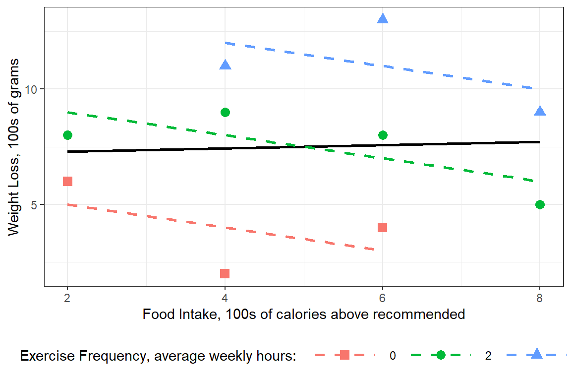
7.3 Regression
GEneric Form
\[ Y_i = b_0 + b_1X_{1i} + b_2X_{2i}+ e_i \]
\[ \hat{Y} = b_0 + b_1X_1 + b_2X_2 \]
fit_lm <- lm(loss ~ exercise + food,
             data = df)

summary(fit_lm)
Call:
lm(formula = loss ~ exercise + food, data = df)

Residuals:
   Min     1Q Median     3Q    Max
    -2     -1      0      1      2

Coefficients:
            Estimate Std. Error t value Pr(>|t|)
(Intercept)   6.0000     1.2749   4.706 0.002193 **
exercise      2.0000     0.3333   6.000 0.000542 ***
food         -0.5000     0.2520  -1.984 0.087623 .
---
Signif. codes:  0 '***' 0.001 '**' 0.01 '*' 0.05 '.' 0.1 ' ' 1

Residual standard error: 1.512 on 7 degrees of freedom
Multiple R-squared:  0.8376,    Adjusted R-squared:  0.7912
F-statistic: 18.05 on 2 and 7 DF,  p-value: 0.001727
\[ \hat{Y} = 6 + 2X_{exercise} -0.5X_{food} \]
Figure 3.5, page 54
effects::Effect(focal.predictors = c("exercise", "food"),
                mod = fit_lm,
                xlevels = list(exercise = c(0, 2, 4))) %>%
  data.frame %>%
  dplyr::mutate(exercise = factor(exercise)) %>%
  ggplot(aes(x = food,
             y = fit,
             fill = exercise)) +
  geom_ribbon(aes(ymin = fit - se,
                  ymax = fit + se),
              alpha = .2) +
  geom_line(aes(color = exercise)) +
  theme_bw() +
  labs(x = "Food Intake, 100s of calories above recommended",
       y = "Weight Loss, 100s of grams",
       fill  = "Exercise Frequency, average weekly hours: ",
       color = "Exercise Frequency, average weekly hours: ") +
  theme(legend.position = "bottom",
legend.key.width = unit(2, "cm")) 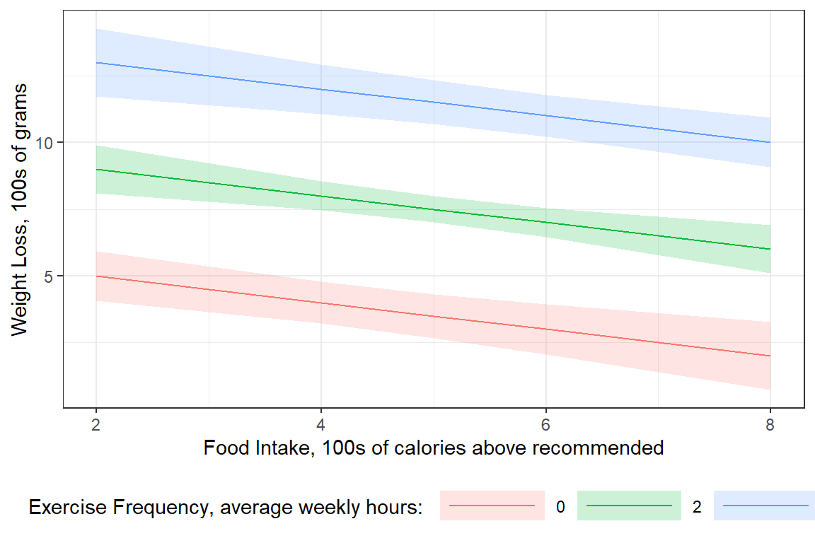
Figrue 3.6, page 54
effects::Effect(focal.predictors = c("exercise", "food"),
                mod = fit_lm,
                xlevels = list(food = c(0, 4,  8))) %>%
  data.frame %>%
  dplyr::mutate(food = factor(food)) %>%
  ggplot(aes(x = exercise,
             y = fit,
             fill = food)) +
  geom_ribbon(aes(ymin = fit - se,
                  ymax = fit + se),
              alpha = .2) +
  geom_line(aes(color = food)) +
  theme_bw() +
  labs(x = "Food Intake, 100s of calories above recommended",
       y = "Exercise Frequency, average weekly hours",
       fill  = "Weight Loss, 100s of grams: ",
       color = "Weight Loss, 100s of grams: ") +
  theme(legend.position = "bottom",
legend.key.width = unit(2, "cm")) 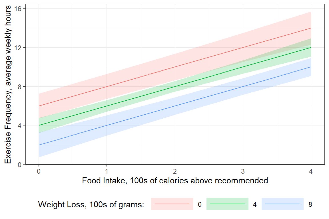
anova(fit_lm)# A tibble: 3 x 5
Df `Sum Sq` `Mean Sq` `F value` `Pr(>F)`
<int> <dbl> <dbl> <dbl> <dbl>
1 1 73.5 73.5 32.2 0.000758
2 1 9 9 3.94 0.0876
3 7 16 2.29 NA NA jtools::summ(fit_lm,
conf = TRUE,
part.corr = TRUE)| Observations | 10 |
| Dependent variable | loss |
| Type | OLS linear regression |
| F(2,7) | 18.05 |
| R² | 0.84 |
| Adj. R² | 0.79 |
| Est. | 2.5% | 97.5% | t val. | p | partial.r | part.r | |
|---|---|---|---|---|---|---|---|
| (Intercept) | 6.00 | 2.99 | 9.01 | 4.71 | 0.00 | NA | NA |
| exercise | 2.00 | 1.21 | 2.79 | 6.00 | 0.00 | 0.91 | 0.91 |
| food | -0.50 | -1.10 | 0.10 | -1.98 | 0.09 | -0.60 | -0.30 |
| Standard errors: OLS |
fit_lm_Z <- lm(scale(loss) ~ scale(exercise) + scale(food),
data = df)summary(fit_lm_Z)
Call:
lm(formula = scale(loss) ~ scale(exercise) + scale(food), data = df)

Residuals:
    Min      1Q  Median      3Q     Max
-0.6046 -0.3023  0.0000  0.3023  0.6046

Coefficients:
                  Estimate Std. Error t value Pr(>|t|)
(Intercept)      8.240e-17  1.445e-01   0.000 1.000000
scale(exercise)  9.872e-01  1.645e-01   6.000 0.000542 ***
scale(food)     -3.265e-01  1.645e-01  -1.984 0.087623 .
---
Signif. codes:  0 '***' 0.001 '**' 0.01 '*' 0.05 '.' 0.1 ' ' 1

Residual standard error: 0.457 on 7 degrees of freedom
Multiple R-squared:  0.8376,    Adjusted R-squared:  0.7912
F-statistic: 18.05 on 2 and 7 DF, p-value: 0.001727texreg::knitreg(list(fit_lm, fit_lm_Z),
single.row = TRUE)| Model 1 | Model 2 | |
|---|---|---|
| (Intercept) | 6.00 (1.27)** | 0.00 (0.14) |
| exercise | 2.00 (0.33)*** | |
| food | -0.50 (0.25) | |
| scale(exercise) | 0.99 (0.16)*** | |
| scale(food) | -0.33 (0.16) | |
| R2 | 0.84 | 0.84 |
| Adj. R2 | 0.79 | 0.79 |
| Num. obs. | 10 | 10 |
| p < 0.001; p < 0.01; p < 0.05 | ||