10 Logistic Regression - Ex: Depression (Hoffman)
library(tidyverse)
library(haven)        # read in SPSS dataset
library(furniture)    # nice table1() descriptives
library(stargazer)    # display nice tables: summary & regression
library(texreg)       # Convert Regression Output to LaTeX or HTML Tables
library(texreghelpr)  # GITHUB: sarbearschartz/texreghelpr
library(psych)        # contains some useful functions, like headTail
library(car)          # Companion to Applied Regression
library(sjPlot)       # Quick plots and tables for models
library(pscl)         # psudo R-squared function
library(glue)         # Interpreted String Literals
library(interactions) # interaction plots
library(sjPlot)       # various plots
library(performance)  # r-squared values
This dataset comes from John Hoffman’s textbook: Regression Models for Categorical, Count, and Related Variables: An Applied Approach (2004) Amazon link, 2014 edition
Chapter 3: Logistic and Probit Regression Models
Dataset: The following example uses the SPSS data set Depress.sav. The dependent variable of interest is a measure of life satisfaction, labeled satlife.
df_depress <- haven::read_spss("https://raw.githubusercontent.com/CEHS-research/data/master/Hoffmann_datasets/depress.sav") %>%
  haven::as_factor()

tibble::glimpse(df_depress)
Rows: 118
Columns: 14
$ id <dbl> 1, 2, 3, 4, 5, 6, 7, 8, 9, 10, 11, 12, 13, 14, 15, 16, 17, 18,~
$ age <dbl> 39, 41, 42, 30, 35, 44, 31, 39, 35, 33, 38, 31, 40, 44, 43, 32~
$ iq <dbl> 94, 89, 83, 99, 94, 90, 94, 87, NA, 92, 92, 94, 91, 86, 90, NA~
$ anxiety <fct> medium low, medium low, medium high, medium low, medium low, N~
$ depress <fct> medium, medium, high, medium, low, low, medium, medium, medium~
$ sleep <fct> low, low, low, low, high, low, NA, low, low, low, high, low, l~
$ sex <fct> female, female, female, female, female, male, female, female, ~
$ lifesat <fct> low, low, low, low, high, high, low, high, low, low, high, hig~
$ weight <dbl> 4.9, 2.2, 4.0, -2.6, -0.3, 0.9, -1.5, 3.5, -1.2, 0.8, -1.9, 5.~
$ satlife <dbl> 0, 0, 0, 0, 1, 1, 0, 1, 0, 0, 1, 1, 1, 0, 0, 1, 1, 0, 0, 1, 0,~
$ male <dbl> 0, 0, 0, 0, 0, 1, 0, 0, 0, 0, 1, 1, 0, 0, 0, 0, 1, 0, 0, 0, 0,~
$ sleep1 <dbl> 0, 0, 0, 0, 1, 0, NA, 0, 0, 0, 1, 0, 0, 0, 0, 1, 0, 0, 0, 0, N~
$ newiq <dbl> 2.21, -2.79, -8.79, 7.21, 2.21, -1.79, 2.21, -4.79, NA, 0.21, ~
$ newage <dbl> 1.5424, 3.5424, 4.5424, -7.4576, -2.4576, 6.5424, -6.4576, 1.5~psych::headTail(df_depress)# A tibble: 9 x 14
id age iq anxiety depress sleep sex lifesat weight satlife male
<chr> <chr> <chr> <fct> <fct> <fct> <fct> <fct> <chr> <chr> <chr>
1 1 39 94 medium low medium low fema~ low 4.9 0 0
2 2 41 89 medium low medium low fema~ low 2.2 0 0
3 3 42 83 medium high high low fema~ low 4 0 0
4 4 30 99 medium low medium low fema~ low -2.6 0 0
5 ... ... ... <NA> <NA> <NA> <NA> <NA> ... ... ...
6 115 39 87 medium low medium low male low <NA> 0 1
7 116 41 86 medium high medium high male low -1 0 1
8 117 33 89 low low high male high 6.5 1 1
9 118 42 <NA> medium high medium low fema~ low 4.9 0 0
# ... with 3 more variables: sleep1 <chr>, newiq <chr>, newage <chr>df_depress %>%
dplyr::select(satlife, lifesat) %>%
table() %>%
addmargins() lifesat
satlife high low Sum
0 0 65 65
1 52 0 52
Sum 52 65 11710.1 Exploratory Data Analysis
Dependent Variable = satlife (numeric version) or lifesat (factor version)
10.1.1 Visualize
df_depress %>%
  ggplot(aes(x = age,
             y = satlife)) +
  geom_count() +
  geom_smooth(method = "lm") +
  theme_bw() +
  labs(x = "Age in Years",
       y = "Life Satisfaction, numeric")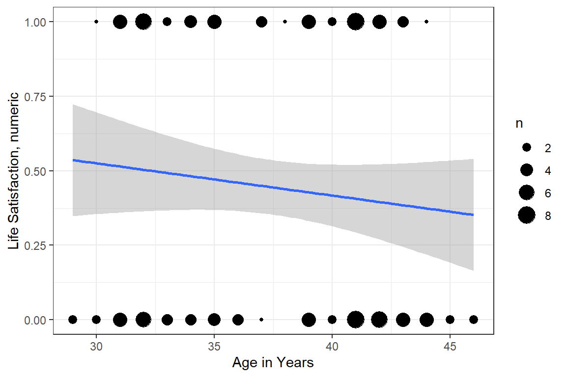
Figure 10.1: Hoffman’s Figure 2.3, top of page 46
df_depress %>%
  ggplot(aes(x = age,
             y = satlife)) +
  geom_count() +
  geom_smooth(method = "lm") +
  theme_bw() +
  labs(x = "Age in Years",
       y = "Life Satisfaction, numeric") +
  facet_grid(~ sex) +
  theme(legend.position = "bottom")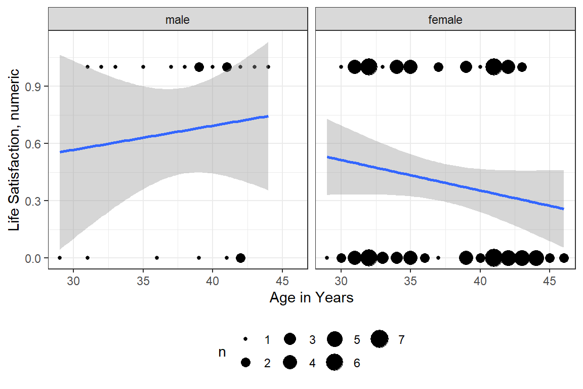
10.1.2 Summary Table
Independent = sex
df_depress %>%
  dplyr::select(lifesat, sex) %>%
  table() %>%
  addmargins()
sex
lifesat male female Sum
high 14 38 52
low 7 58 65
Sum 21 96 117df_depress %>%
dplyr::group_by(sex) %>%
furniture::table1(lifesat,
total = TRUE,
caption = "Hoffman's EXAMPLE 3.1 Cross-Tabulation of Gender and Life Satisfaction (top page 50)",
output = "markdown")| Total | male | female | |
|---|---|---|---|
| n = 117 | n = 21 | n = 96 | |
| lifesat | |||
| high | 52 (44.4%) | 14 (66.7%) | 38 (39.6%) |
| low | 65 (55.6%) | 7 (33.3%) | 58 (60.4%) |
10.2 Calcualte: Probability, Odds, and Odds-Ratios
10.2.1 Marginal, over all the sample
Tally the number of participants happy and not happy (i.e. depressed).
df_depress %>%
  dplyr::select(satlife) %>%
  table() %>%
  addmargins()
.
0 1 Sum
65 52 117 10.2.1.1 Probability of being happy
\[ prob_{yes} = \frac{n_{yes}}{n_{total}} = \frac{n_{yes}}{n_{yes} + n_{no}} \]
prob <- 52 / 117

prob
[1] 0.444444410.2.1.2 Odds of being happy
\[ odds_{yes} = \frac{n_{yes}}{n_{no}} = \frac{n_{yes}}{n_{total} - n_{yes}} \]
odds <- 52/65

odds
[1] 0.8\[ odds_{yes} = \frac{prob_{yes}}{prob_{no}} = \frac{prob_{yes}}{1 - prob_{yes}} \]
prob/(1 - prob)[1] 0.810.2.2 Comparing by Sex
Cross-tabulate happiness (
satlife) withsex(male vs. female).
df_depress %>%
  dplyr::select(satlife, sex) %>%
  table() %>%
  addmargins()
sex
satlife male female Sum
0 7 58 65
1 14 38 52
Sum 21 96 11710.2.2.1 Probability of being happy, by sex
Reference category = male
prob_male <- 14 / 21

prob_male
[1] 0.6666667Comparison Category = female
prob_female <- 38 / 96

prob_female
[1] 0.395833310.2.2.2 Odds of being happy, by sex
Reference category = male
odds_male <- 14 / 7

odds_male
[1] 2Comparison Category = female
odds_female <- 38 / 58


odds_female
[1] 0.655172410.2.2.3 Odds-Ratio for sex
\[ OR_{\text{female vs. male}} = \frac{odds_{female}}{odds_{male}} \]
odds_ratio <- odds_female / odds_male

odds_ratio
[1] 0.3275862\[ OR_{\text{female vs. male}} = \frac{\frac{prob_{female}}{1 - prob_{female}}}{\frac{prob_{male}}{1 - prob_{male}}} \]
(prob_female / (1 - prob_female)) / (prob_male / (1 - prob_male))[1] 0.3275862\[ OR_{\text{female vs. male}} = \frac{\frac{n_{yes|female}}{n_{no|female}}}{\frac{n_{yes|male}}{n_{no|male}}} \]
((38 / 58)/(14 / 7))[1] 0.327586210.3 Logisitc Regression Model 1: one IV
10.3.1 Fit the Unadjusted Model
fit_glm_1 <- glm(satlife ~ sex,
                 data = df_depress,
                 family = binomial(link = "logit"))

fit_glm_1 %>% summary() %>% coef()
Estimate Std. Error z value Pr(>|z|)
(Intercept) 0.6931472 0.4629100 1.497369 0.13429719
sexfemale -1.1160040 0.5077822 -2.197800 0.02796333summary(fit_glm_1)
Call:
glm(formula = satlife ~ sex, family = binomial(link = "logit"),
    data = df_depress)

Deviance Residuals:
   Min      1Q  Median      3Q     Max
-1.482  -1.004  -1.004   1.361   1.361

Coefficients:
            Estimate Std. Error z value Pr(>|z|)
(Intercept)   0.6931     0.4629   1.497    0.134
sexfemale    -1.1160     0.5078  -2.198    0.028 *
---
Signif. codes:  0 '***' 0.001 '**' 0.01 '*' 0.05 '.' 0.1 ' ' 1

(Dispersion parameter for binomial family taken to be 1)

    Null deviance: 160.75  on 116  degrees of freedom
Residual deviance: 155.62  on 115  degrees of freedom
  (1 observation deleted due to missingness)
AIC: 159.62

Number of Fisher Scoring iterations: 4
10.3.2 Tabulate Parameters
10.3.2.1 Logit Scale
texreg::knitreg(fit_glm_1,
                caption = "Hoffman's EXAMPLE 3.2 A Loistic Regression Model of Gender and Life Satisfaction, top of page 51",
                caption.above = TRUE,
                single.row = TRUE,
digits = 4)| Model 1 | |
|---|---|
| (Intercept) | 0.6931 (0.4629) |
| sexfemale | -1.1160 (0.5078)* |
| AIC | 159.6205 |
| BIC | 165.1449 |
| Log Likelihood | -77.8103 |
| Deviance | 155.6205 |
| Num. obs. | 117 |
| p < 0.001; p < 0.01; p < 0.05 | |
10.3.2.2 Both Logit and Odds-ratio Scales
texreg::knitreg(list(fit_glm_1,
                     texreghelpr::extract_glm_exp(fit_glm_1)),
                custom.model.names = c("b (SE)",
                                       "OR [95 CI]"),
                caption = "Hoffman's EXAMPLE 3.2 A Loistic Regression Model of Gender and Life Satisfaction, top of page 51",
                caption.above = TRUE,
                single.row = TRUE,
                digits = 4,
ci.test = 1)| b (SE) | OR [95 CI] | |
|---|---|---|
| (Intercept) | 0.6931 (0.4629) | 2.0000 [0.8322; 5.2772] |
| sexfemale | -1.1160 (0.5078)* | 0.3276 [0.1148; 0.8625]* |
| AIC | 159.6205 | |
| BIC | 165.1449 | |
| Log Likelihood | -77.8103 | |
| Deviance | 155.6205 | |
| Num. obs. | 117 | |
| p < 0.001; p < 0.01; p < 0.05 (or Null hypothesis value outside the confidence interval). | ||
10.3.3 Assess Model Fit
10.3.3.1 Likelihood Ratio Test (LRT, aka. Deviance Difference Test)
drop1(fit_glm_1, test = "LRT")# A tibble: 2 x 5
Df Deviance AIC LRT `Pr(>Chi)`
<dbl> <dbl> <dbl> <dbl> <dbl>
1 NA 156. 160. NA NA
2 1 161. 163. 5.13 0.0235performance::compare_performance(fit_glm_1)# A tibble: 1 x 11
Name Model AIC BIC R2_Tjur RMSE Sigma Log_loss Score_log Score_spherical
<chr> <chr> <dbl> <dbl> <dbl> <dbl> <dbl> <dbl> <dbl> <dbl>
1 fit_glm_1 glm 160. 165. 0.0437 0.486 1.16 0.665 -30.1 0.0550
# ... with 1 more variable: PCP <dbl>10.3.3.2 R-squared “like” measures
performance::r2(fit_glm_1)# R2 for Logistic Regression
Tjur's R2: 0.044performance::r2_mcfadden(fit_glm_1)# R2 for Generalized Linear Regression
R2: 0.032
adj. R2: 0.019performance::r2_nagelkerke(fit_glm_1)Nagelkerke's R2
0.05742029 pscl::pR2(fit_glm_1)fitting null model for pseudo-r2 llh llhNull G2 McFadden r2ML r2CU
-77.81025523 -80.37450446 5.12849846 0.03190376 0.04288652 0.05742029 10.3.4 Plot Predicted Probabilitites
sjPlot::plot_model(model = fit_glm_1,
                   type = "pred")
$sex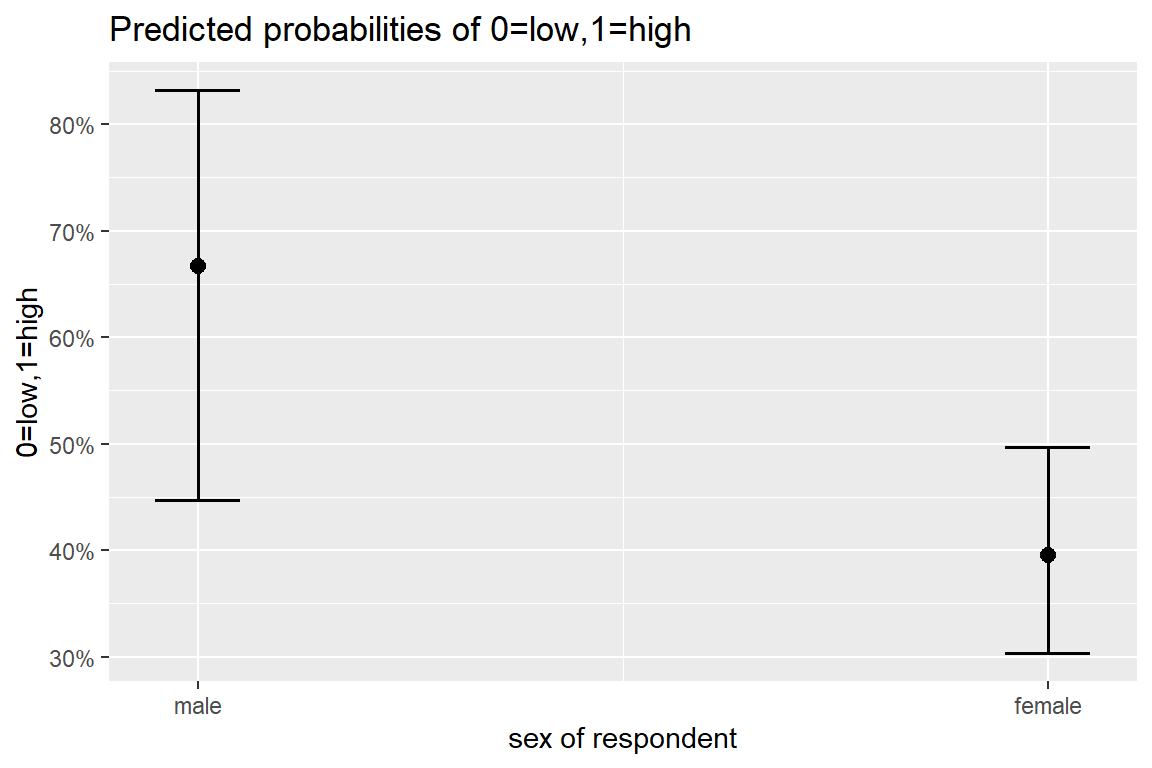
10.3.4.1 Logit scale
fit_glm_1 %>%
  emmeans::emmeans(~ sex)
sex emmean SE df asymp.LCL asymp.UCL
male 0.693 0.463 Inf -0.214 1.6004
female -0.423 0.209 Inf -0.832 -0.0138
Results are given on the logit (not the response) scale.
Confidence level used: 0.95 fit_glm_1 %>%
emmeans::emmeans(~ sex) %>%
pairs() contrast estimate SE df z.ratio p.value
male - female 1.12 0.508 Inf 2.198 0.0280
Results are given on the log odds ratio (not the response) scale. 10.3.4.2 Response Scale (probability)
fit_glm_1 %>%
  emmeans::emmeans(~ sex,
                   type = "response")
sex prob SE df asymp.LCL asymp.UCL
male 0.667 0.1029 Inf 0.447 0.832
female 0.396 0.0499 Inf 0.303 0.497
Confidence level used: 0.95
Intervals are back-transformed from the logit scale fit_glm_1 %>%
emmeans::emmeans(~ sex,
type = "response") %>%
pairs() contrast odds.ratio SE df null z.ratio p.value
male / female 3.05 1.55 Inf 1 2.198 0.0280
Tests are performed on the log odds ratio scale 10.3.5 Interpretation
On average, two out of every three males is depressed, b = 0.667, odds = 1.95, 95% CI [1.58, 2.40].
Females have nearly a quarter lower odds of being depressed, compared to men, b = -0.27, OR = 0.77, 95% IC [0.61, 0.96], p = .028.
10.3.6 Diagnostics
10.3.6.1 Influential values
Influential values are extreme individual data points that can alter the quality of the logistic regression model.
The most extreme values in the data can be examined by visualizing the Cook’s distance values. Here we label the top 7 largest values:
plot(fit_glm_1, which = 4, id.n = 7)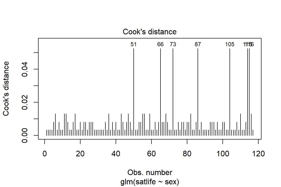
Note that, not all outliers are influential observations. To check whether the data contains potential influential observations, the standardized residual error can be inspected. Data points with an absolute standardized residuals above 3 represent possible outliers and may deserve closer attention.
10.3.6.2 Standardized Residuals
The following R code computes the standardized residuals (.std.resid) using the R function augment() [broom package].
fit_glm_1 %>%
  broom::augment() %>%
  ggplot(aes(x = .rownames, .std.resid)) +
  geom_point(aes(color = sex), alpha = .5) +
  theme_bw()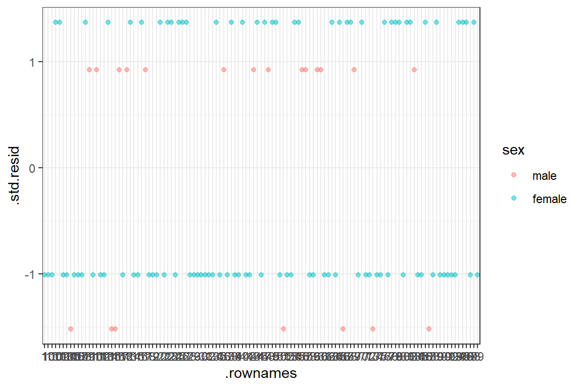
10.4 Logisitic Regression Model 2: many IV’s
10.4.1 Fit the Model
fit_glm_2 <- glm(satlife ~ sex + iq + age + weight,
                 data = df_depress,
                 family = binomial(link = "logit"))

fit_glm_2 %>% summary() %>% coef()
Estimate Std. Error z value Pr(>|z|)
(Intercept) 9.02054236 6.01858970 1.4987801 0.13393069
sexfemale -1.27924381 0.55971456 -2.2855289 0.02228183
iq -0.07279837 0.05361036 -1.3579161 0.17449031
age -0.04112838 0.05250052 -0.7833900 0.43339814
weight -0.03768972 0.08885942 -0.4241499 0.6714564810.4.2 Tabulate Parameters
texreg::knitreg(list(fit_glm_2,
                     texreghelpr::extract_glm_exp(fit_glm_2)),
                custom.model.names = c("b (SE)",
                                       "OR [95 CI]"),
                caption = "EXAMPLE 3.3 A Logistic Regression Model of Life Satisfaction with Multiple Independent Variables, middle of page 52",
                caption.above = TRUE,
                single.row = TRUE,
                digits = 4,
ci.test = 1)| b (SE) | OR [95 CI] | |
|---|---|---|
| (Intercept) | 9.0205 (6.0186) | 8271.2619 [0.0854; 2077566352.1374] |
| sexfemale | -1.2792 (0.5597)* | 0.2782 [0.0870; 0.8060]* |
| iq | -0.0728 (0.0536) | 0.9298 [0.8327; 1.0304] |
| age | -0.0411 (0.0525) | 0.9597 [0.8635; 1.0627] |
| weight | -0.0377 (0.0889) | 0.9630 [0.8073; 1.1472] |
| AIC | 137.5217 | |
| BIC | 150.4973 | |
| Log Likelihood | -63.7609 | |
| Deviance | 127.5217 | |
| Num. obs. | 99 | |
| p < 0.001; p < 0.01; p < 0.05 (or Null hypothesis value outside the confidence interval). | ||
10.4.3 Assess Model Fit
drop1(fit_glm_2, test = "LRT")# A tibble: 5 x 5
Df Deviance AIC LRT `Pr(>Chi)`
<dbl> <dbl> <dbl> <dbl> <dbl>
1 NA 128. 138. NA NA
2 1 133. 141. 5.59 0.0180
3 1 129. 137. 1.91 0.167
4 1 128. 136. 0.621 0.431
5 1 128. 136. 0.180 0.671 10.4.4 Variance Explained
performance::compare_performance(fit_glm_2)# A tibble: 1 x 11
Name Model AIC BIC R2_Tjur RMSE Sigma Log_loss Score_log Score_spherical
<chr> <chr> <dbl> <dbl> <dbl> <dbl> <dbl> <dbl> <dbl> <dbl>
1 fit_glm_2 glm 138. 150. 0.0753 0.475 1.16 0.644 -23.1 0.0220
# ... with 1 more variable: PCP <dbl>10.4.4.1 R-squared “lik” measures
performance::r2_nagelkerke(fit_glm_2)Nagelkerke's R2
0.09728404 10.4.5 Diagnostics
10.4.5.1 Multicollinearity
Multicollinearity corresponds to a situation where the data contain highly correlated predictor variables. Read more in Chapter (ref?)(multicollinearity).
Multicollinearity is an important issue in regression analysis and should be fixed by removing the concerned variables. It can be assessed using the R function vif() [car package], which computes the variance inflation factors:
car::vif(fit_glm_2) sex iq age weight
1.011608 1.294334 1.418975 1.233364 As a rule of thumb, a VIF value that exceeds 5 or 10 indicates a problematic amount of collinearity. In our example, there is no collinearity: all variables have a value of VIF well below 5.
10.5 Compare Models
10.5.1 Refit to Complete Cases
Restrict the data to only participant that have all four of these predictors.
df_depress_model <- df_depress %>%
                        dplyr::filter(complete.cases(sex, iq, age, weight))
Refit Model 1 with only participant complete on all the predictors.
fit_glm_1_redo <- glm(satlife ~ sex,
                      data = df_depress_model,
                      family = binomial(link = "logit"))

fit_glm_2_redo <- glm(satlife ~ sex + iq + age + weight,
                      data = df_depress_model,
family = binomial(link = "logit"))texreg::knitreg(list(texreghelpr::extract_glm_exp(fit_glm_1_redo),
texreghelpr::extract_glm_exp(fit_glm_2_redo)),
custom.model.names = c("Single IV",
"Multiple IVs"),
caption.above = TRUE,
single.row = TRUE,
digits = 4,
ci.test = 1)| Single IV | Multiple IVs | |
|---|---|---|
| (Intercept) | 2.0000 [0.7767; 5.7449] | 8271.2619 [0.0854; 2077566352.1374] |
| sexfemale | 0.2941 [0.0939; 0.8387]* | 0.2782 [0.0870; 0.8060]* |
| iq | 0.9298 [0.8327; 1.0304] | |
| age | 0.9597 [0.8635; 1.0627] | |
| weight | 0.9630 [0.8073; 1.1472] | |
| * Null hypothesis value outside the confidence interval. | ||
anova(fit_glm_1_redo,
      fit_glm_2_redo,
      test = "LRT")
# A tibble: 2 x 5
`Resid. Df` `Resid. Dev` Df Deviance `Pr(>Chi)`
<dbl> <dbl> <dbl> <dbl> <dbl>
1 97 130. NA NA NA
2 94 128. 3 2.18 0.537performance::compare_performance(fit_glm_1_redo,
fit_glm_2_redo,
rank = TRUE)# A tibble: 2 x 12
Name Model AIC BIC R2_Tjur RMSE Sigma Log_loss Score_log Score_spherical
<chr> <chr> <dbl> <dbl> <dbl> <dbl> <dbl> <dbl> <dbl> <dbl>
1 fit_glm_1_redo glm 134. 139. 0.0535 0.481 1.16 0.655 -22.8 0.0591
2 fit_glm_2_redo glm 138. 150. 0.0753 0.475 1.16 0.644 -23.1 0.0220
# ... with 2 more variables: PCP <dbl>, Performance_Score <dbl>10.5.2 Interpretation
- Only sex is predictive of depression. There is no evidence IQ, age, or weight are associated with depression, all p’s > .16.
10.6 Changing the reference category
df_depress$sex [1] female female female female female male female female female female
[11] male male female female female female male female female female
[21] female female female female female female female female female female
[31] female female female female female male female female female female
[41] female female male female female female female male female female
[51] male female female female female male male female female male
[61] female female female female female male female female male female
[71] female female male female female female female female female female
[81] female female male female female female male female female female
[91] female female female female female female female female female female
[101] female female female female male female female female female female
[111] male female female female male male male female
attr(,"label")
[1] sex of respondent
Levels: male femaledf_depress_ref <- df_depress %>%
dplyr::mutate(male = sex %>% forcats::fct_relevel("female", after = 0))
df_depress_ref$male [1] female female female female female male female female female female
[11] male male female female female female male female female female
[21] female female female female female female female female female female
[31] female female female female female male female female female female
[41] female female male female female female female male female female
[51] male female female female female male male female female male
[61] female female female female female male female female male female
[71] female female male female female female female female female female
[81] female female male female female female male female female female
[91] female female female female female female female female female female
[101] female female female female male female female female female female
[111] male female female female male male male female
attr(,"label")
[1] sex of respondent
Levels: female malefit_glm_2_male <- glm(satlife ~ male + iq + age + weight,
data = df_depress,
family = binomial(link = "logit"))texreg::knitreg(list(texreghelpr::extract_glm_exp(fit_glm_2),
texreghelpr::extract_glm_exp(fit_glm_2_male)),
custom.model.names = c("original model",
"recoded model"),
caption.above = TRUE,
single.row = TRUE,
digits = 4,
ci.test = 1)| original model | recoded model | |
|---|---|---|
| (Intercept) | 8271.2619 [0.0854; 2077566352.1374] | 2301.4590 [0.0263; 482461590.3668] |
| sexfemale | 0.2782 [0.0870; 0.8060]* | |
| iq | 0.9298 [0.8327; 1.0304] | 0.9298 [0.8327; 1.0304] |
| age | 0.9597 [0.8635; 1.0627] | 0.9597 [0.8635; 1.0627] |
| weight | 0.9630 [0.8073; 1.1472] | 0.9630 [0.8073; 1.1472] |
| male | 3.5939 [1.2406; 11.4938]* | |
| * Null hypothesis value outside the confidence interval. | ||