9 Logistic Regression - Ex: Maternal Risk Factor for Low Birth Weight Delivery
library(tidyverse)
library(haven)        # read in SPSS dataset
library(furniture)    # nice table1() descriptives
library(stargazer)    # display nice tables: summary & regression
library(texreg)       # Convert Regression Output to LaTeX or HTML Tables
library(texreghelpr)  #
library(psych)        # contains some useful functions, like headTail
library(car)          # Companion to Applied Regression
library(sjPlot)       # Quick plots and tables for models
library(pscl)         # psudo R-squared function
library(glue)         # Interpreted String Literals
library(interactions) # interaction plots
library(sjPlot)       # various plots
library(performance)  # r-squared values
9.1 Background
More complex example demonstrating modeling decisions
Another set of data from a study investigating predictors of low birth weight
idinfant’s unique identification number
Dependent variable (DV) or outcome
lowLow birth weight (outcome)- 0 = birth weight >2500 g (normal)
- 1 = birth weight < 2500 g (low))
bwtactual infant birth weight in grams (ignore for now)
Independent variables (IV) or predictors
ageAge of mother, in yearslwtMother’s weight at last menstrual period, in poundsraceRace: 1 = White, 2 = Black, 3 = OthersmokeSmoking status during pregnancy:1 = Yes, 0 = NoptlHistory of premature labor: 0 = None, 1 = One, 2 = two, 3 = threehtHistory of hypertension: 1 = Yes, 0 = NouiUterine irritability: 1 = Yes, 0 = NoftvNumber of physician visits in 1st trimester: 0 = None, 1 = One, … 6 = six
9.1.1 Raw Dataset
The data is saved in a text file (.txt) without any labels.
lowbwt_raw <- read.table("https://raw.githubusercontent.com/CEHS-research/data/master/Regression/lowbwt.txt",
                         header = TRUE,
                         sep = "",
                         na.strings = "NA",
                         dec = ".",
                         strip.white = TRUE)

tibble::glimpse(lowbwt_raw)
Rows: 189
Columns: 11
$ id <int> 85, 86, 87, 88, 89, 91, 92, 93, 94, 95, 96, 97, 98, 99, 100, 101~
$ low <int> 0, 0, 0, 0, 0, 0, 0, 0, 0, 0, 0, 0, 0, 0, 0, 0, 0, 0, 0, 0, 0, 0~
$ age <int> 19, 33, 20, 21, 18, 21, 22, 17, 29, 26, 19, 19, 22, 30, 18, 18, ~
$ lwt <int> 182, 155, 105, 108, 107, 124, 118, 103, 123, 113, 95, 150, 95, 1~
$ race <int> 2, 3, 1, 1, 1, 3, 1, 3, 1, 1, 3, 3, 3, 3, 1, 1, 2, 1, 3, 1, 3, 1~
$ smoke <int> 0, 0, 1, 1, 1, 0, 0, 0, 1, 1, 0, 0, 0, 0, 1, 1, 0, 1, 0, 1, 0, 0~
$ ptl <int> 0, 0, 0, 0, 0, 0, 0, 0, 0, 0, 0, 0, 0, 1, 0, 0, 0, 0, 0, 0, 0, 0~
$ ht <int> 0, 0, 0, 0, 0, 0, 0, 0, 0, 0, 0, 0, 1, 0, 0, 0, 0, 0, 0, 0, 0, 0~
$ ui <int> 1, 0, 0, 1, 1, 0, 0, 0, 0, 0, 0, 0, 0, 1, 0, 0, 0, 0, 1, 0, 0, 1~
$ ftv <int> 0, 3, 1, 2, 0, 0, 1, 1, 1, 0, 0, 1, 0, 2, 0, 0, 0, 3, 0, 1, 2, 3~
$ bwt <int> 2523, 2551, 2557, 2594, 2600, 2622, 2637, 2637, 2663, 2665, 2722~9.1.2 Declare Factors
lowbwt_clean <- lowbwt_raw %>%
  dplyr::mutate(id = factor(id)) %>%
  dplyr::mutate(low = low %>%
                  factor() %>%
                  forcats::fct_recode("birth weight >2500 g (normal)" = "0",
                                      "birth weight < 2500 g (low)"   = "1")) %>%
  dplyr::mutate(race = race %>%
                  factor() %>%
                  forcats::fct_recode("White" = "1",
                                      "Black" = "2",
                                      "Other" = "3")) %>%
  dplyr::mutate(ptl_any = as.numeric(ptl > 0)) %>%         # collapse into 0 = none vs. 1 = at least one
  dplyr::mutate(ptl = factor(ptl)) %>%                     # declare the number of pre-term labors to be a factor: 0, 1, 2, 3
  dplyr::mutate_at(vars(smoke, ht, ui, ptl_any),           # declare all there variables to be factors with the same two levels
                   factor,
                   levels = 0:1,
                   labels = c("No", "Yes"))
Display the structure of the ‘clean’ version of the dataset
tibble::glimpse(lowbwt_clean)Rows: 189
Columns: 12
$ id <fct> 85, 86, 87, 88, 89, 91, 92, 93, 94, 95, 96, 97, 98, 99, 100, 1~
$ low <fct> birth weight >2500 g (normal), birth weight >2500 g (normal), ~
$ age <int> 19, 33, 20, 21, 18, 21, 22, 17, 29, 26, 19, 19, 22, 30, 18, 18~
$ lwt <int> 182, 155, 105, 108, 107, 124, 118, 103, 123, 113, 95, 150, 95,~
$ race <fct> Black, Other, White, White, White, Other, White, Other, White,~
$ smoke <fct> No, No, Yes, Yes, Yes, No, No, No, Yes, Yes, No, No, No, No, Y~
$ ptl <fct> 0, 0, 0, 0, 0, 0, 0, 0, 0, 0, 0, 0, 0, 1, 0, 0, 0, 0, 0, 0, 0,~
$ ht <fct> No, No, No, No, No, No, No, No, No, No, No, No, Yes, No, No, N~
$ ui <fct> Yes, No, No, Yes, Yes, No, No, No, No, No, No, No, No, Yes, No~
$ ftv <int> 0, 3, 1, 2, 0, 0, 1, 1, 1, 0, 0, 1, 0, 2, 0, 0, 0, 3, 0, 1, 2,~
$ bwt <int> 2523, 2551, 2557, 2594, 2600, 2622, 2637, 2637, 2663, 2665, 27~
$ ptl_any <fct> No, No, No, No, No, No, No, No, No, No, No, No, No, Yes, No, N~lowbwt_clean# A tibble: 189 x 12
id low age lwt race smoke ptl ht ui ftv bwt ptl_any
<fct> <fct> <int> <int> <fct> <fct> <fct> <fct> <fct> <int> <int> <fct>
1 85 birth we~ 19 182 Black No 0 No Yes 0 2523 No
2 86 birth we~ 33 155 Other No 0 No No 3 2551 No
3 87 birth we~ 20 105 White Yes 0 No No 1 2557 No
4 88 birth we~ 21 108 White Yes 0 No Yes 2 2594 No
5 89 birth we~ 18 107 White Yes 0 No Yes 0 2600 No
6 91 birth we~ 21 124 Other No 0 No No 0 2622 No
7 92 birth we~ 22 118 White No 0 No No 1 2637 No
8 93 birth we~ 17 103 Other No 0 No No 1 2637 No
9 94 birth we~ 29 123 White Yes 0 No No 1 2663 No
10 95 birth we~ 26 113 White Yes 0 No No 0 2665 No
# ... with 179 more rows9.2 Exploratory Data Analysis
lowbwt_clean %>%
  furniture::table1("Age, years" = age,
                    "Weight, pounds" = lwt,
                    "Race" = race,
                    "Smoking During pregnancy" = smoke,
                    "History of Premature Labor, any" = ptl_any,
                    "History of Premature Labor, number" = ptl,
                    "History of Hypertension" = ht,
                    "Uterince Irritability" = ui,
                    "1st Tri Dr Visits" = ftv,
                    splitby = ~ low,
                    test = TRUE,
output = "markdown")| birth weight >2500 g (normal) | birth weight < 2500 g (low) | P-Value | |
|---|---|---|---|
| n = 130 | n = 59 | ||
| Age, years | 0.103 | ||
| 23.7 (5.6) | 22.3 (4.5) | ||
| Weight, pounds | 0.02 | ||
| 133.3 (31.7) | 122.1 (26.6) | ||
| Race | 0.082 | ||
| White | 73 (56.2%) | 23 (39%) | |
| Black | 15 (11.5%) | 11 (18.6%) | |
| Other | 42 (32.3%) | 25 (42.4%) | |
| Smoking During pregnancy | 0.04 | ||
| No | 86 (66.2%) | 29 (49.2%) | |
| Yes | 44 (33.8%) | 30 (50.8%) | |
| History of Premature Labor, any | <.001 | ||
| No | 118 (90.8%) | 41 (69.5%) | |
| Yes | 12 (9.2%) | 18 (30.5%) | |
| History of Premature Labor, number | <.001 | ||
| 0 | 118 (90.8%) | 41 (69.5%) | |
| 1 | 8 (6.2%) | 16 (27.1%) | |
| 2 | 3 (2.3%) | 2 (3.4%) | |
| 3 | 1 (0.8%) | 0 (0%) | |
| History of Hypertension | 0.076 | ||
| No | 125 (96.2%) | 52 (88.1%) | |
| Yes | 5 (3.8%) | 7 (11.9%) | |
| Uterince Irritability | 0.035 | ||
| No | 116 (89.2%) | 45 (76.3%) | |
| Yes | 14 (10.8%) | 14 (23.7%) | |
| 1st Tri Dr Visits | 0.389 | ||
| 0.8 (1.1) | 0.7 (1.0) |
9.3 Logistic Regression - Simple, unadjusted models
low1.age   <- glm(low ~ age,     family = binomial(link = "logit"), data = lowbwt_clean)
low1.lwt   <- glm(low ~ lwt,     family = binomial(link = "logit"), data = lowbwt_clean)
low1.race  <- glm(low ~ race,    family = binomial(link = "logit"), data = lowbwt_clean)
low1.smoke <- glm(low ~ smoke,   family = binomial(link = "logit"), data = lowbwt_clean)
low1.ptl   <- glm(low ~ ptl_any, family = binomial(link = "logit"), data = lowbwt_clean)
low1.ht    <- glm(low ~ ht,      family = binomial(link = "logit"), data = lowbwt_clean)
low1.ui    <- glm(low ~ ui,      family = binomial(link = "logit"), data = lowbwt_clean)
low1.ftv   <- glm(low ~ ftv,     family = binomial(link = "logit"), data = lowbwt_clean)
Note: the parameter estimates here are for the LOGIT scale, not the odds ration (OR) or even the probability.
texreg::knitreg(list(low1.age, low1.lwt, low1.race, low1.smoke),
                custom.model.names = c("Age", "Weight", "Race", "Smoker"),
                caption = "Simple, Unadjusted Logistic Regression: Models 1-4",
                caption.above = TRUE,
digits = 3)| Age | Weight | Race | Smoker | |
|---|---|---|---|---|
| (Intercept) | 0.385 | 0.998 | -1.155*** | -1.087*** |
| (0.732) | (0.785) | (0.239) | (0.215) | |
| age | -0.051 | |||
| (0.032) | ||||
| lwt | -0.014* | |||
| (0.006) | ||||
| raceBlack | 0.845 | |||
| (0.463) | ||||
| raceOther | 0.636 | |||
| (0.348) | ||||
| smokeYes | 0.704* | |||
| (0.320) | ||||
| AIC | 235.912 | 232.691 | 235.662 | 233.805 |
| BIC | 242.395 | 239.174 | 245.387 | 240.288 |
| Log Likelihood | -115.956 | -114.345 | -114.831 | -114.902 |
| Deviance | 231.912 | 228.691 | 229.662 | 229.805 |
| Num. obs. | 189 | 189 | 189 | 189 |
| p < 0.001; p < 0.01; p < 0.05 | ||||
texreg::knitreg(list(low1.ptl, low1.ht, low1.ui, low1.ftv),
                custom.model.names = c("Pre-Labor", "Hypertension", "Uterine", "Visits"),
                caption = "Simple, Unadjusted Logistic Regression: Models 5-8",
                caption.above = TRUE,
digits = 3)| Pre-Labor | Hypertension | Uterine | Visits | |
|---|---|---|---|---|
| (Intercept) | -1.057*** | -0.877*** | -0.947*** | -0.687*** |
| (0.181) | (0.165) | (0.176) | (0.195) | |
| ptl_anyYes | 1.463*** | |||
| (0.414) | ||||
| htYes | 1.214* | |||
| (0.608) | ||||
| uiYes | 0.947* | |||
| (0.417) | ||||
| ftv | -0.135 | |||
| (0.157) | ||||
| AIC | 225.898 | 234.650 | 233.596 | 237.899 |
| BIC | 232.381 | 241.133 | 240.079 | 244.382 |
| Log Likelihood | -110.949 | -115.325 | -114.798 | -116.949 |
| Deviance | 221.898 | 230.650 | 229.596 | 233.899 |
| Num. obs. | 189 | 189 | 189 | 189 |
| p < 0.001; p < 0.01; p < 0.05 | ||||
9.4 Logistic Regression - Multivariate, with Main Effects Only
Main-effects multiple logistic regression model
low1_1 <- glm(low ~ age + lwt + race + smoke + ptl_any + ht + ui,
              family = binomial(link = "logit"),
              data = lowbwt_clean)

summary(low1_1)
Call:
glm(formula = low ~ age + lwt + race + smoke + ptl_any + ht +
    ui, family = binomial(link = "logit"), data = lowbwt_clean)

Deviance Residuals:
    Min       1Q   Median       3Q      Max
-1.6459  -0.7992  -0.5103   0.9388   2.2018

Coefficients:
            Estimate Std. Error z value Pr(>|z|)
(Intercept)  0.63691    1.23028   0.518  0.60467
age         -0.03775    0.03781  -0.998  0.31808
lwt         -0.01491    0.00704  -2.118  0.03419 *
raceBlack    1.21274    0.53248   2.278  0.02275 *
raceOther    0.80412    0.44843   1.793  0.07294 .
smokeYes     0.84640    0.40806   2.074  0.03806 *
ptl_anyYes   1.22175    0.46301   2.639  0.00832 **
htYes        1.83869    0.70324   2.615  0.00893 **
uiYes        0.71113    0.46311   1.536  0.12465
---
Signif. codes:  0 '***' 0.001 '**' 0.01 '*' 0.05 '.' 0.1 ' ' 1

(Dispersion parameter for binomial family taken to be 1)

    Null deviance: 234.67  on 188  degrees of freedom
Residual deviance: 196.83  on 180  degrees of freedom
AIC: 214.83

Number of Fisher Scoring iterations: 4
9.5 Logistic Regression - Multivariate, with Interactions
Before removing non-significant main effects, test plausible interactions
Try interactions between age and lwt, age and smoke, lwt and smoke, 1 at a time
9.5.1 Age and Weight
low1_2 <- glm(low ~ age + lwt + race + smoke + ptl_any + ht + ui + age:lwt,
                 family = binomial(link = "logit"),
                 data = lowbwt_clean)

summary(low1_2)
Call:
glm(formula = low ~ age + lwt + race + smoke + ptl_any + ht +
    ui + age:lwt, family = binomial(link = "logit"), data = lowbwt_clean)

Deviance Residuals:
    Min       1Q   Median       3Q      Max
-1.6426  -0.8004  -0.5163   0.9400   2.1989

Coefficients:
              Estimate Std. Error z value Pr(>|z|)
(Intercept)  1.1396293  4.0443041   0.282  0.77811
age         -0.0597273  0.1724339  -0.346  0.72906
lwt         -0.0188377  0.0309225  -0.609  0.54240
raceBlack    1.2071359  0.5341716   2.260  0.02383 *
raceOther    0.7977750  0.4505381   1.771  0.07661 .
smokeYes     0.8433655  0.4083953   2.065  0.03892 *
ptl_anyYes   1.2260463  0.4642795   2.641  0.00827 **
htYes        1.8389418  0.7034162   2.614  0.00894 **
uiYes        0.7142688  0.4642468   1.539  0.12391
age:lwt      0.0001718  0.0013146   0.131  0.89600
---
Signif. codes:  0 '***' 0.001 '**' 0.01 '*' 0.05 '.' 0.1 ' ' 1

(Dispersion parameter for binomial family taken to be 1)

    Null deviance: 234.67  on 188  degrees of freedom
Residual deviance: 196.82  on 179  degrees of freedom
AIC: 216.82

Number of Fisher Scoring iterations: 5
9.5.1.1 Compare Model Fits vs. Likelihood Ratio Test
anova(low1_1, low1_2, test = 'LRT')# A tibble: 2 x 5
`Resid. Df` `Resid. Dev` Df Deviance `Pr(>Chi)`
<dbl> <dbl> <dbl> <dbl> <dbl>
1 180 197. NA NA NA
2 179 197. 1 0.0170 0.8969.5.1.2 Type II Analysis of Deviance Table
Anova(low1_2, test = 'LR') # A tibble: 8 x 3
`LR Chisq` Df `Pr(>Chisq)`
<dbl> <dbl> <dbl>
1 1.02 1 0.313
2 5.00 1 0.0254
3 6.27 2 0.0436
4 4.38 1 0.0364
5 7.13 1 0.00758
6 7.18 1 0.00738
7 2.33 1 0.127
8 0.0170 1 0.896 9.5.1.3 Type III Analysis of Deviance Table
Anova(low1_2, test = 'LR', type = 'III') # A tibble: 8 x 3
`LR Chisq` Df `Pr(>Chisq)`
<dbl> <dbl> <dbl>
1 0.119 1 0.730
2 0.372 1 0.542
3 6.27 2 0.0436
4 4.38 1 0.0364
5 7.13 1 0.00758
6 7.18 1 0.00738
7 2.33 1 0.127
8 0.0170 1 0.896 9.5.2 Age and Smoking
low1_3 <- glm(low ~ age + lwt + race + smoke + ptl_any + ht + ui + age:smoke,
                 family = binomial(link = "logit"),
                 data = lowbwt_clean)

summary(low1_3)
Call:
glm(formula = low ~ age + lwt + race + smoke + ptl_any + ht +
    ui + age:smoke, family = binomial(link = "logit"), data = lowbwt_clean)

Deviance Residuals:
    Min       1Q   Median       3Q      Max
-1.7020  -0.8016  -0.4970   0.9055   2.2124

Coefficients:
              Estimate Std. Error z value Pr(>|z|)
(Intercept)   1.311029   1.483078   0.884  0.37670
age          -0.068293   0.053865  -1.268  0.20485
lwt          -0.014701   0.007001  -2.100  0.03575 *
raceBlack     1.126482   0.543684   2.072  0.03827 *
raceOther     0.768241   0.451199   1.703  0.08863 .
smokeYes     -0.601286   1.782234  -0.337  0.73583
ptl_anyYes    1.197295   0.460992   2.597  0.00940 **
htYes         1.860851   0.705311   2.638  0.00833 **
uiYes         0.783999   0.472451   1.659  0.09703 .
age:smokeYes  0.063744   0.076634   0.832  0.40552
---
Signif. codes:  0 '***' 0.001 '**' 0.01 '*' 0.05 '.' 0.1 ' ' 1

(Dispersion parameter for binomial family taken to be 1)

    Null deviance: 234.67  on 188  degrees of freedom
Residual deviance: 196.14  on 179  degrees of freedom
AIC: 216.14

Number of Fisher Scoring iterations: 5
9.5.2.1 Compare Model Fits vs. Likelihood Ratio Test
anova(low1_1, low1_3, test = 'LRT')# A tibble: 2 x 5
`Resid. Df` `Resid. Dev` Df Deviance `Pr(>Chi)`
<dbl> <dbl> <dbl> <dbl> <dbl>
1 180 197. NA NA NA
2 179 196. 1 0.699 0.403performance::compare_performance(low1_1, low1_3, rank = TRUE)# A tibble: 2 x 12
Name Model AIC BIC R2_Tjur RMSE Sigma Log_loss Score_log Score_spherical
<chr> <chr> <dbl> <dbl> <dbl> <dbl> <dbl> <dbl> <dbl> <dbl>
1 low1_1 glm 215. 244. 0.190 0.418 1.05 0.521 -24.6 0.0164
2 low1_3 glm 216. 249. 0.192 0.417 1.05 0.519 -24.5 0.0156
# ... with 2 more variables: PCP <dbl>, Performance_Score <dbl>9.5.3 Weight and Smoking
low1_4 <- glm(low ~ age + lwt + race + smoke + ptl_any + ht + ui + lwt:smoke,
                 family = binomial(link = "logit"),
                 data = lowbwt_clean)

summary(low1_4)
Call:
glm(formula = low ~ age + lwt + race + smoke + ptl_any + ht +
    ui + lwt:smoke, family = binomial(link = "logit"), data = lowbwt_clean)

Deviance Residuals:
    Min       1Q   Median       3Q      Max
-1.6816  -0.7874  -0.5251   0.8876   2.2365

Coefficients:
             Estimate Std. Error z value Pr(>|z|)
(Intercept)   1.74840    1.59439   1.097  0.27282
age          -0.03768    0.03809  -0.989  0.32259
lwt          -0.02362    0.01077  -2.193  0.02828 *
raceBlack     1.23110    0.53358   2.307  0.02104 *
raceOther     0.71646    0.45183   1.586  0.11281
smokeYes     -1.13566    1.75557  -0.647  0.51770
ptl_anyYes    1.26472    0.46488   2.721  0.00652 **
htYes         1.74326    0.70738   2.464  0.01373 *
uiYes         0.80121    0.47044   1.703  0.08855 .
lwt:smokeYes  0.01555    0.01344   1.157  0.24740
---
Signif. codes:  0 '***' 0.001 '**' 0.01 '*' 0.05 '.' 0.1 ' ' 1

(Dispersion parameter for binomial family taken to be 1)

    Null deviance: 234.67  on 188  degrees of freedom
Residual deviance: 195.44  on 179  degrees of freedom
AIC: 215.44

Number of Fisher Scoring iterations: 5
9.5.3.1 Compare Model Fits vs. Likelihood Ratio Test
anova(low1_1, low1_4, test = 'LRT')# A tibble: 2 x 5
`Resid. Df` `Resid. Dev` Df Deviance `Pr(>Chi)`
<dbl> <dbl> <dbl> <dbl> <dbl>
1 180 197. NA NA NA
2 179 195. 1 1.39 0.2389.6 Logistic Regression - Multivariate, Simplify
No interactions are significant Remove non-significant main effects
9.6.1 Remove the least significant perdictor: ui
low1_5 <- glm(low ~ age + lwt + race + smoke + ptl_any + ht,
                 family = binomial(link = "logit"),
                 data = lowbwt_clean)

summary(low1_5)
Call:
glm(formula = low ~ age + lwt + race + smoke + ptl_any + ht,
    family = binomial(link = "logit"), data = lowbwt_clean)

Deviance Residuals:
    Min       1Q   Median       3Q      Max
-1.6533  -0.8202  -0.5299   0.9709   2.1982

Coefficients:
             Estimate Std. Error z value Pr(>|z|)
(Intercept)  0.924910   1.202693   0.769  0.44187
age         -0.042784   0.037567  -1.139  0.25475
lwt         -0.015436   0.007044  -2.191  0.02843 *
raceBlack    1.168452   0.532577   2.194  0.02824 *
raceOther    0.814620   0.442740   1.840  0.06578 .
smokeYes     0.858332   0.404787   2.120  0.03397 *
ptl_anyYes   1.333970   0.457573   2.915  0.00355 **
htYes        1.740511   0.703104   2.475  0.01331 *
---
Signif. codes:  0 '***' 0.001 '**' 0.01 '*' 0.05 '.' 0.1 ' ' 1

(Dispersion parameter for binomial family taken to be 1)

    Null deviance: 234.67  on 188  degrees of freedom
Residual deviance: 199.15  on 181  degrees of freedom
AIC: 215.15

Number of Fisher Scoring iterations: 4
9.7 Logistic Regression - Multivariate, Final Model
Since the mother’s age is theoretically a meaningful variable, it should probably be retained.
Revise so that age is interpreted in 5-year and lwt in 20 lb increments and the intercept has meaning.
low1_6 <- glm(low ~ I((age - 20)/5) + I((lwt - 125)/20) + race + smoke + ptl_any + ht,
              family = binomial(link = "logit"),
              data = lowbwt_clean)

summary(low1_6)
Call:
glm(formula = low ~ I((age - 20)/5) + I((lwt - 125)/20) + race +
    smoke + ptl_any + ht, family = binomial(link = "logit"),
    data = lowbwt_clean)

Deviance Residuals:
    Min       1Q   Median       3Q      Max
-1.6533  -0.8202  -0.5299   0.9709   2.1982

Coefficients:
                  Estimate Std. Error z value Pr(>|z|)
(Intercept)        -1.8603     0.4092  -4.546 5.48e-06 ***
I((age - 20)/5)    -0.2139     0.1878  -1.139  0.25475
I((lwt - 125)/20)  -0.3087     0.1409  -2.191  0.02843 *
raceBlack           1.1685     0.5326   2.194  0.02824 *
raceOther           0.8146     0.4427   1.840  0.06578 .
smokeYes            0.8583     0.4048   2.120  0.03397 *
ptl_anyYes          1.3340     0.4576   2.915  0.00355 **
htYes               1.7405     0.7031   2.475  0.01331 *
---
Signif. codes:  0 '***' 0.001 '**' 0.01 '*' 0.05 '.' 0.1 ' ' 1

(Dispersion parameter for binomial family taken to be 1)

    Null deviance: 234.67  on 188  degrees of freedom
Residual deviance: 199.15  on 181  degrees of freedom
AIC: 215.15

Number of Fisher Scoring iterations: 4
9.7.1 Several \(R^2\) measures with the pscl::pR2() function
pscl::pR2(low1_6)fitting null model for pseudo-r2 llh llhNull G2 McFadden r2ML r2CU
-99.5757045 -117.3359981 35.5205871 0.1513627 0.1713353 0.2409463 performance::r2(low1_6)# R2 for Logistic Regression
Tjur's R2: 0.1809.7.2 Parameter Estiamtes Table
9.7.2.1 Using texreg::screenreg()
Default: parameters are in terms of the ‘logit’ or log odds ratio
texreg::knitreg(low1_6,
                single.row = TRUE,
digits = 3)| Model 1 | |
|---|---|
| (Intercept) | -1.860 (0.409)*** |
| (age - 20)/5 | -0.214 (0.188) |
| (lwt - 125)/20 | -0.309 (0.141)* |
| raceBlack | 1.168 (0.533)* |
| raceOther | 0.815 (0.443) |
| smokeYes | 0.858 (0.405)* |
| ptl_anyYes | 1.334 (0.458)** |
| htYes | 1.741 (0.703)* |
| AIC | 215.151 |
| BIC | 241.085 |
| Log Likelihood | -99.576 |
| Deviance | 199.151 |
| Num. obs. | 189 |
| p < 0.001; p < 0.01; p < 0.05 | |
The texreg package uses an intermediate function called extract() to extract information for the model and then put it in the right places in the table. I have writen a function called extract_glm_exp() that is helpful.
texreg::knitreg(extract_glm_exp(low1_6),
                  custom.coef.names = c("BL: 125 lb, 20 yr old White Mother",
                                        "Additional 5 years older",
                                        "Additional 20 lbs pre-pregnancy",
                                        "Race: Black vs. White",
                                        "Race: Other vs. White",
                                        "Smoking During pregnancy",
                                        "History of Any Premature Labor",
                                        "History of Hypertension"),
                  custom.model.names = "OR, Low Birth Weight",
                  single.row = TRUE,
ci.test = 1)| OR, Low Birth Weight | |
|---|---|
| BL: 125 lb, 20 yr old White Mother | 0.16 [0.07; 0.33]* |
| Additional 5 years older | 0.81 [0.55; 1.16] |
| Additional 20 lbs pre-pregnancy | 0.73 [0.55; 0.95]* |
| Race: Black vs. White | 3.22 [1.13; 9.31]* |
| Race: Other vs. White | 2.26 [0.96; 5.50] |
| Smoking During pregnancy | 2.36 [1.08; 5.32]* |
| History of Any Premature Labor | 3.80 [1.57; 9.53]* |
| History of Hypertension | 5.70 [1.49; 24.76]* |
| * 1 outside the confidence interval. | |
texreg::knitreg(list(low1_6,
                     extract_glm_exp(low1_6,
                                     include.aic = FALSE,
                                     include.bic = FALSE,
                                     include.loglik = FALSE,
                                     include.deviance = FALSE,
                                     include.nobs = FALSE)),
                custom.model.names = c("b (SE)",
                                       "OR [95 CI]"),
                custom.coef.map = list("(Intercept)" = "BL: 125 lb, 20 yr old White Mother",
                                    "I((age - 20)/5)" = "Additional 5 years older",
                                    "I((lwt - 125)/20)" = "Additional 20 lbs pre-pregnancy",
                                    "raceBlack" = "Race: Black vs. White",
                                    "raceOther" = "Race: Other vs. White",
                                    "smokeYes" = "Smoking During pregnancy",
                                    "ptl_anyYes" = "History of Any Premature Labor",
                                    "htYes" = "History of Hypertension"),
                caption = "Maternal Factors effect Low Birthweight of Infant",
                caption.above = TRUE,
                single.row = TRUE,
ci.test = 1)| b (SE) | OR [95 CI] | |
|---|---|---|
| BL: 125 lb, 20 yr old White Mother | -1.86 (0.41)*** | 0.16 [0.07; 0.33]* |
| Additional 5 years older | -0.21 (0.19) | 0.81 [0.55; 1.16] |
| Additional 20 lbs pre-pregnancy | -0.31 (0.14)* | 0.73 [0.55; 0.95]* |
| Race: Black vs. White | 1.17 (0.53)* | 3.22 [1.13; 9.31]* |
| Race: Other vs. White | 0.81 (0.44) | 2.26 [0.96; 5.50] |
| Smoking During pregnancy | 0.86 (0.40)* | 2.36 [1.08; 5.32]* |
| History of Any Premature Labor | 1.33 (0.46)** | 3.80 [1.57; 9.53]* |
| History of Hypertension | 1.74 (0.70)* | 5.70 [1.49; 24.76]* |
| AIC | 215.15 | |
| BIC | 241.09 | |
| Log Likelihood | -99.58 | |
| Deviance | 199.15 | |
| Num. obs. | 189 | |
| p < 0.001; p < 0.01; p < 0.05 (or Null hypothesis value outside the confidence interval). | ||
9.7.3 Marginal Model Plot
9.7.3.1 Focus on: Mother’s Age, weight, and race
interactions::interact_plot(model = low1_6,
                            pred = lwt,
                            modx = race,
                            mod2 = age)
effects::Effect(focal.predictors = c("age", "lwt", "race"),
                mod = low1_6,
                xlevels = list(age = c(20, 30, 40),
                               lwt = seq(from = 80, to = 250, by = 5))) %>%
  data.frame() %>%
  dplyr::mutate(age_labels = glue("Mother Age: {age}")) %>%
  ggplot(aes(x = lwt,
             y = fit)) +
  geom_line(aes(color = race,
                linetype = race),
            size = 1) +
  theme_bw() +
  facet_grid(.~ age_labels) +
  labs(title = "Risk of Low Birth Weight",
       subtitle = "Illustates risk given mother is a non-smoker, without a history of pre-term labor or hypertension",
       x = "Mother's Weight Pre-Pregnancy, pounds",
       y = "Predicted Probability\nBaby has Low Birth Weight (< 2500 grams)",
       color    = "Mother's Race",
       linetype = "Mother's Race") +
  theme(legend.position = c(1, 1),
        legend.justification = c(1.1, 1.1),
        legend.background = element_rect(color = "black"),
        legend.key.width = unit(2, "cm")) +
  scale_linetype_manual(values = c("longdash", "dotted", "solid")) +
  scale_color_manual(values = c( "coral2", "dodger blue", "gray50"))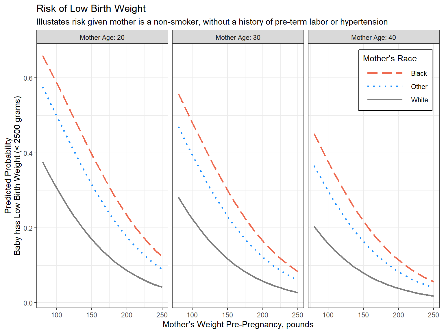
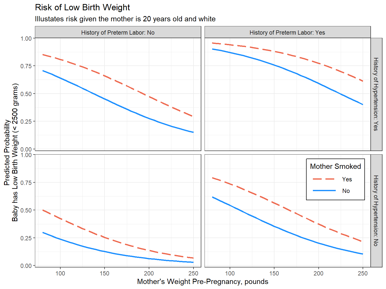
9.7.3.2 Focus on: Mother’s weight and smoking status during pregnancy, as well as history of any per-term labor and hypertension
interactions::interact_plot(model = low1_6,
                            pred = lwt,
                            modx = smoke,
                            mod2 = ptl_any)
interactions::interact_plot(model = low1_6,
                            pred = lwt,
                            modx = smoke,
                            mod2 = ht)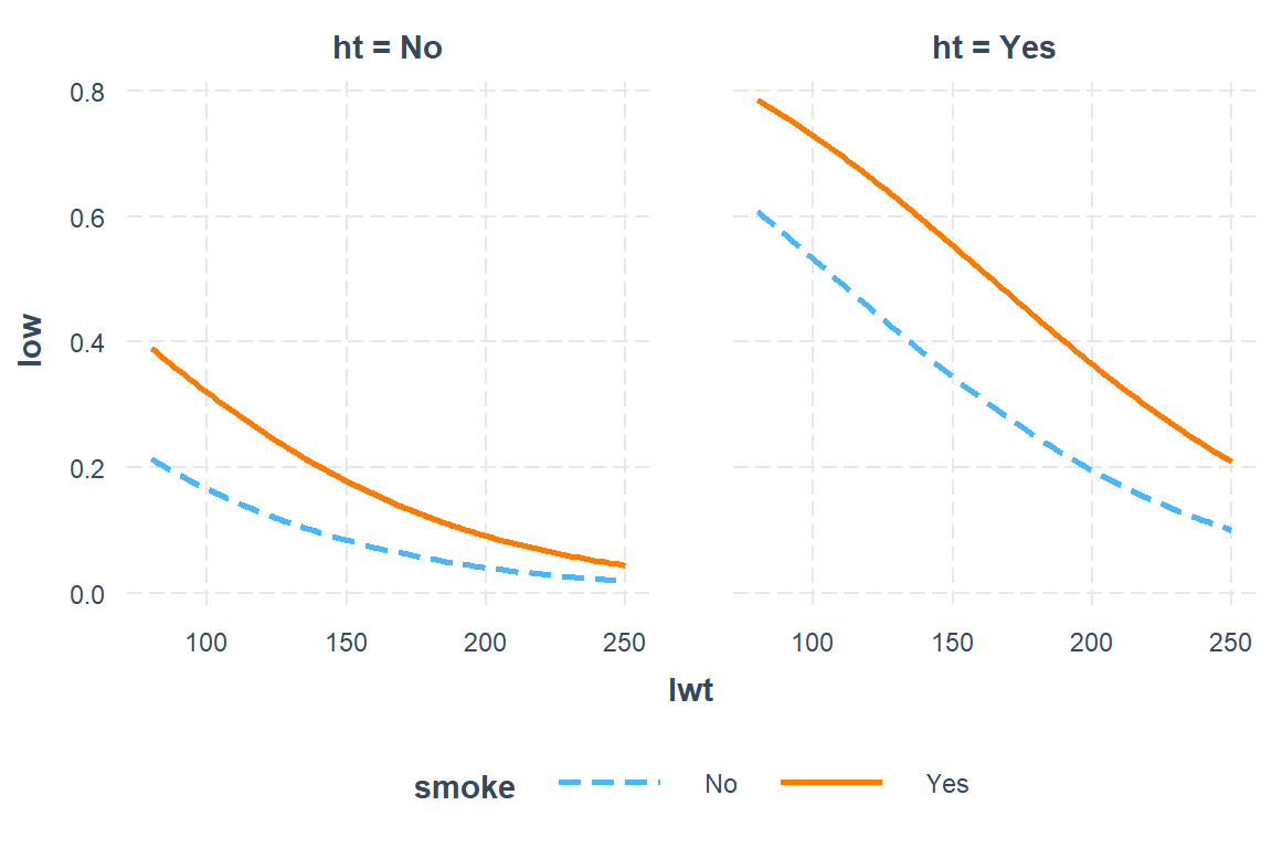
effects::Effect(focal.predictors = c("lwt", "smoke", "ptl_any", "ht"),
                fixed.predictors = list(age = 20),
                mod = low1_6,
                xlevels = list(lwt = seq(from = 80, to = 250, by = 5))) %>%
  data.frame() %>%
  dplyr::mutate(smoke = forcats::fct_rev(smoke)) %>%
  dplyr::mutate(ptl_any_labels = glue("History of Preterm Labor: {ptl_any}")) %>%
  dplyr::mutate(ht_labels = glue("History of Hypertension: {ht}") %>% forcats::fct_rev()) %>%
  ggplot(aes(x = lwt,
             y = fit)) +
  geom_line(aes(color = smoke,
                linetype = smoke),
            size = 1) +
  theme_bw() +
  facet_grid(ht_labels ~ ptl_any_labels) +
  labs(title = "Risk of Low Birth Weight",
       subtitle = "Illustates risk given the mother is 20 years old and white",
       x = "Mother's Weight Pre-Pregnancy, pounds",
       y = "Predicted Probability\nBaby has Low Birth Weight (< 2500 grams)",
       color    = "Mother Smoked",
       linetype = "Mother Smoked") +
  theme(legend.position = c(1, .5),
        legend.justification = c(1.1, 1.15),
        legend.background = element_rect(color = "black"),
        legend.key.width = unit(1.5, "cm")) +
  scale_linetype_manual(values = c("longdash", "solid")) +
  scale_color_manual(values = c( "coral2", "dodger blue"))