2 Simple Linear Regression - Example: Cancer Experiment
2.1 Background
2.1.1 Required Packages
library(tidyverse)    # Loads several very helpful 'tidy' packages
library(haven)        # Read in SPSS datasets
library(psych)        # Lots of nice tid-bits
library(GGally)       # Extension to 'ggplot2' (ggpairs)
2.1.2 Example Dataset - Cancer Experiment
The Cancer dataset:
cancer_raw <- haven::read_spss("https://raw.githubusercontent.com/CEHS-research/eBook_ANOVA/master/data/Cancer.sav")

tibble::glimpse(cancer_raw)
Rows: 25
Columns: 9
$ ID <dbl> 1, 5, 6, 9, 11, 15, 21, 26, 31, 35, 39, 41, 45, 2, 12, 14, 16~
$ TRT <dbl> 0, 0, 0, 0, 0, 0, 0, 0, 0, 0, 0, 0, 0, 0, 1, 1, 1, 1, 1, 1, 1~
$ AGE <dbl> 52, 77, 60, 61, 59, 69, 67, 56, 61, 51, 46, 65, 67, 46, 56, 4~
$ WEIGHIN <dbl> 124.0, 160.0, 136.5, 179.6, 175.8, 167.6, 186.0, 158.0, 212.8~
$ STAGE <dbl> 2, 1, 4, 1, 2, 1, 1, 3, 1, 1, 4, 1, 1, 2, 4, 1, 2, 1, 4, 2, 1~
$ TOTALCIN <dbl> 6, 9, 7, 6, 6, 6, 6, 6, 6, 6, 7, 6, 8, 7, 6, 4, 6, 6, 12, 5, ~
$ TOTALCW2 <dbl> 6, 6, 9, 7, 7, 6, 11, 11, 9, 4, 8, 6, 8, 16, 10, 6, 11, 7, 11~
$ TOTALCW4 <dbl> 6, 10, 17, 9, 16, 6, 11, 15, 6, 8, 11, 9, 9, 9, 11, 8, 11, 6,~
$ TOTALCW6 <dbl> 7, 9, 19, 3, 13, 11, 10, 15, 8, 7, 11, 6, 10, 10, 9, 7, 14, 6~cancer_clean <- cancer_raw %>%
dplyr::rename_all(tolower) %>%
dplyr::mutate(id = factor(id)) %>%
dplyr::mutate(trt = factor(trt,
labels = c("Placebo",
"Aloe Juice"))) %>%
dplyr::mutate(stage = factor(stage))
tibble::glimpse(cancer_clean)Rows: 25
Columns: 9
$ id <fct> 1, 5, 6, 9, 11, 15, 21, 26, 31, 35, 39, 41, 45, 2, 12, 14, 16~
$ trt <fct> Placebo, Placebo, Placebo, Placebo, Placebo, Placebo, Placebo~
$ age <dbl> 52, 77, 60, 61, 59, 69, 67, 56, 61, 51, 46, 65, 67, 46, 56, 4~
$ weighin <dbl> 124.0, 160.0, 136.5, 179.6, 175.8, 167.6, 186.0, 158.0, 212.8~
$ stage <fct> 2, 1, 4, 1, 2, 1, 1, 3, 1, 1, 4, 1, 1, 2, 4, 1, 2, 1, 4, 2, 1~
$ totalcin <dbl> 6, 9, 7, 6, 6, 6, 6, 6, 6, 6, 7, 6, 8, 7, 6, 4, 6, 6, 12, 5, ~
$ totalcw2 <dbl> 6, 6, 9, 7, 7, 6, 11, 11, 9, 4, 8, 6, 8, 16, 10, 6, 11, 7, 11~
$ totalcw4 <dbl> 6, 10, 17, 9, 16, 6, 11, 15, 6, 8, 11, 9, 9, 9, 11, 8, 11, 6,~
$ totalcw6 <dbl> 7, 9, 19, 3, 13, 11, 10, 15, 8, 7, 11, 6, 10, 10, 9, 7, 14, 6~psych::headTail(cancer_clean)# A tibble: 9 x 9
id trt age weighin stage totalcin totalcw2 totalcw4 totalcw6
<fct> <fct> <chr> <chr> <fct> <chr> <chr> <chr> <chr>
1 1 Placebo 52 124 2 6 6 6 7
2 5 Placebo 77 160 1 9 6 10 9
3 6 Placebo 60 136.5 4 7 9 17 19
4 9 Placebo 61 179.6 1 6 7 9 3
5 <NA> <NA> ... ... <NA> ... ... ... ...
6 42 Aloe Juice 73 181.5 0 8 11 16 <NA>
7 44 Aloe Juice 67 187 1 5 7 7 7
8 50 Aloe Juice 60 164 2 6 8 16 <NA>
9 58 Aloe Juice 54 172.8 4 7 8 10 8 2.2 Exploratory Data Analysis: i.e. the eyeball method
2.2.1 Scatterplot
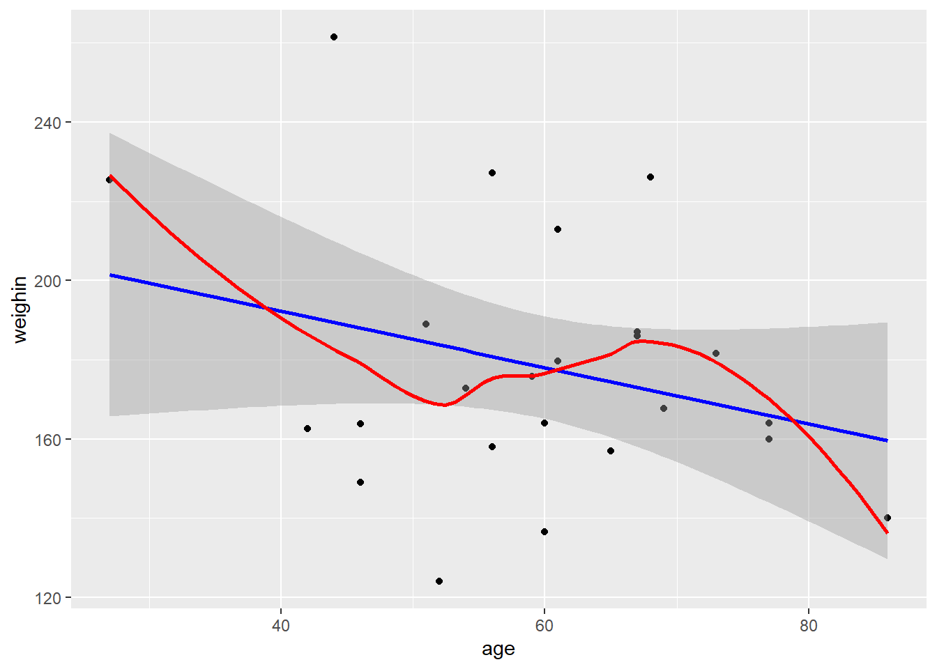
Always plot your data first!
cancer_clean %>%
  ggplot(aes(x = age,
             y = weighin)) +
  geom_point() +
  geom_smooth(method = "lm",    se = TRUE,  color = "blue") +  # straight line (linear model)
  geom_smooth(method = "loess", se = FALSE, color = "red")     # loess line (moving window)