10 Binomial Sign Test

library(tidyverse)
library(pander)

10.1 The Binomial Distribution

data.frame(count = 0:13) %>% 
  dplyr::mutate(prob = dbinom(count, size = 13, p = .50)) %>% 
  ggplot(aes(x = count,
             y = prob)) +
  geom_point() +
  geom_segment(aes(xend = count, 
                   y = 0, 
                   yend = prob),
               size = .1) +
  theme_bw() +
  scale_x_continuous() +
  labs(x = "Count",
       y = "Probability") +
  theme(legend.position = "none")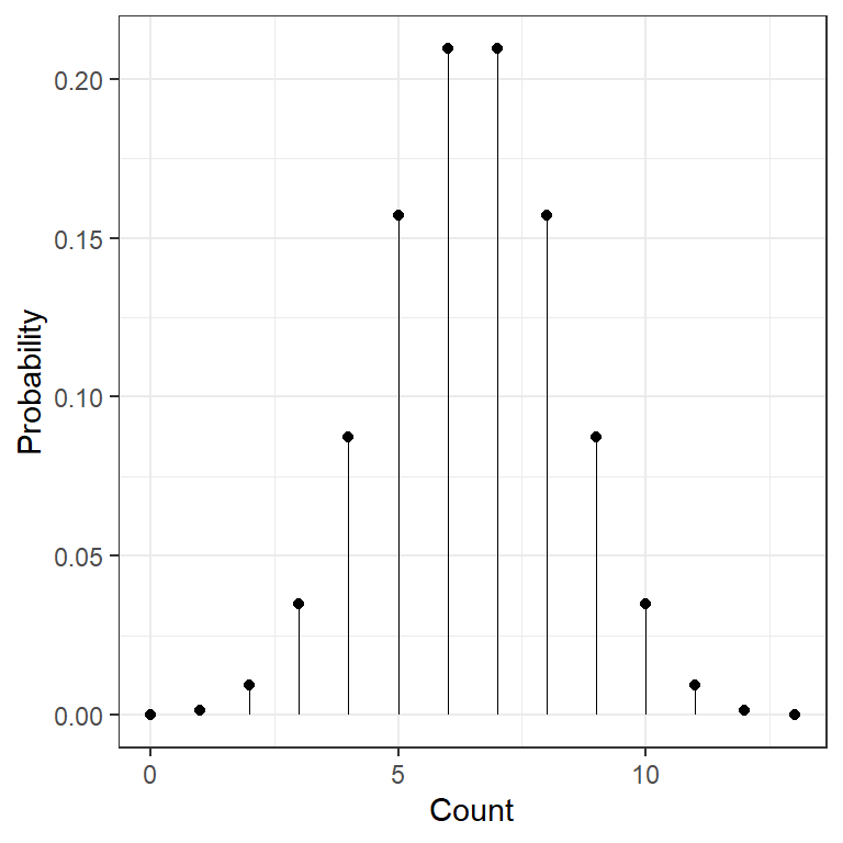

10.1.1 Effect of Hypothesised “P” Value

ex_n = 30

data.frame(count = 0:35) %>% 
  dplyr::mutate(prob_10 = dbinom(count, size = ex_n, p = .10)) %>% 
  dplyr::mutate(prob_25 = dbinom(count, size = ex_n, p = .25)) %>% 
  dplyr::mutate(prob_50 = dbinom(count, size = ex_n, p = .50)) %>% 
  dplyr::mutate(prob_75 = dbinom(count, size = ex_n, p = .75)) %>% 
  dplyr::mutate(prob_90 = dbinom(count, size = ex_n, p = .90)) %>%
  tidyr::pivot_longer(cols = contains("prob"),
                      names_to = "percent",
                      names_prefix = "prob_",
                      values_to = "prob") %>% 
  dplyr::mutate(percent = paste0("P = .", percent)) %>% 
  ggplot(aes(x = count,
             y = prob)) +
  geom_point() +
  geom_segment(aes(xend = count, 
                   y = 0, 
                   yend = prob),
               size = .1) +
  theme_bw() +
  scale_x_continuous() +
  labs(x = "Count",
       y = "Probability") +
  theme(legend.position = "none") +
  facet_grid(~ percent)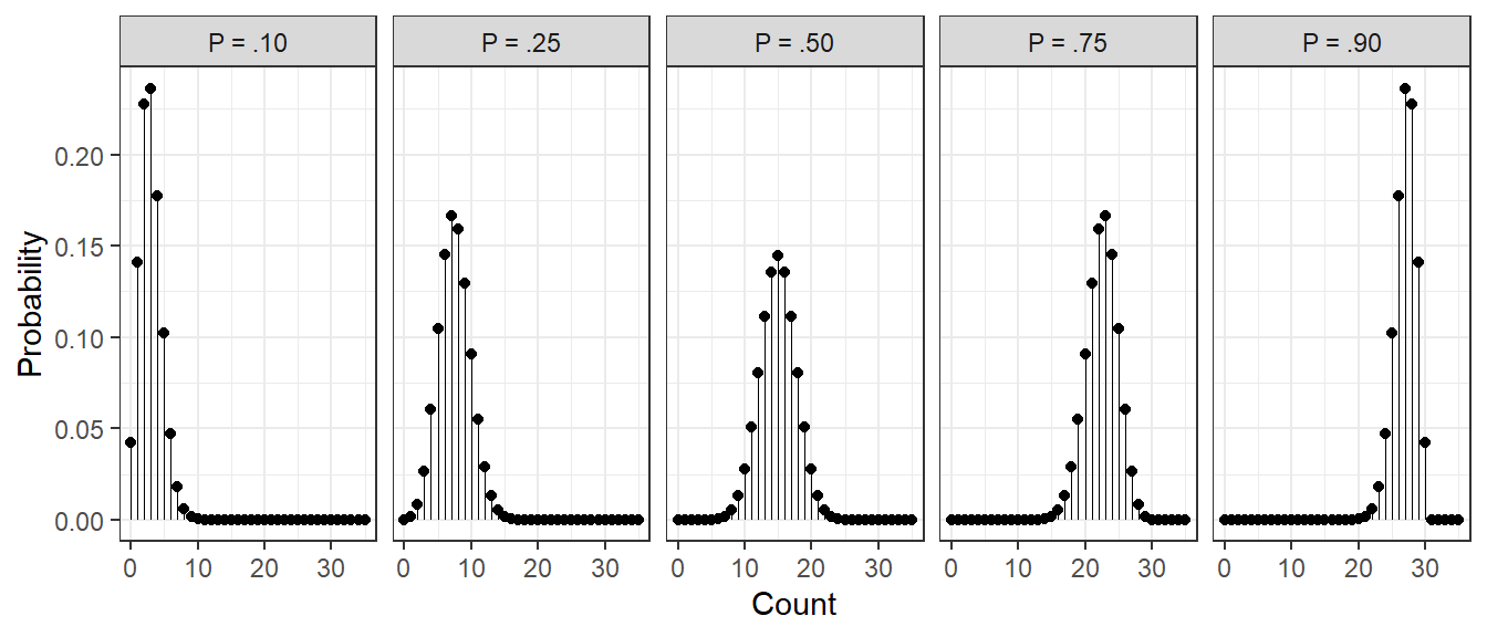

10.1.2 Effect of Sample Size

10.1.3 Probability of 4 (or more) out of 5

ex_n = 5
ex_x = 4
ex_p = .50

dbinom(x    = ex_x, 
       size = ex_n, 
       prob = ex_p)

[1] 0.15625

data.frame(count = 0:ex_n) %>% 
  dplyr::mutate(prob = dbinom(count, size = ex_n, p = ex_p)) %>% 
  dplyr::mutate(mark = cut(count, 
                           breaks = c(0, ex_x - .5, ex_n),
                           include.lowest = TRUE)) %>% 
  ggplot(aes(x = count,
             y = prob,
             color = mark)) +
  geom_point(size = 2) +
  geom_segment(aes(xend = count, 
                   y = 0, 
                   yend = prob),
               size = 1) +
  theme_bw() +
  scale_x_continuous(breaks = 0:ex_n) +
  scale_color_manual(values = c("black", "red")) +
  labs(x = "Count",
       y = "Probability") +
  theme(legend.position = "none")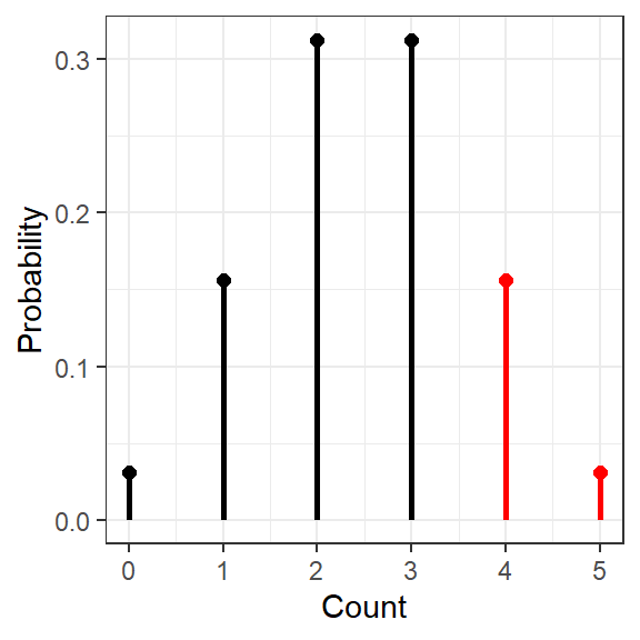

10.1.4 Probability of 8 (or more) out of 10

ex_n = 10
ex_x = 8
ex_p = .50

dbinom(x    = ex_x, 
       size = ex_n, 
       prob = ex_p)

[1] 0.04394531

data.frame(count = 0:ex_n) %>% 
  dplyr::mutate(prob = dbinom(count, size = ex_n, p = ex_p)) %>% 
  dplyr::mutate(mark = cut(count, 
                           breaks = c(0, ex_x -.5, ex_n),
                           include.lowest = TRUE)) %>% 
  ggplot(aes(x = count,
             y = prob,
             color = mark)) +
  geom_point(size = 2) +
  geom_segment(aes(xend = count, 
                   y = 0, 
                   yend = prob),
               size = 1) +
  theme_bw() +
  scale_x_continuous(breaks = 0:ex_n) +
  scale_color_manual(values = c("black", "red")) +
  labs(x = "Count",
       y = "Probability") +
  theme(legend.position = "none")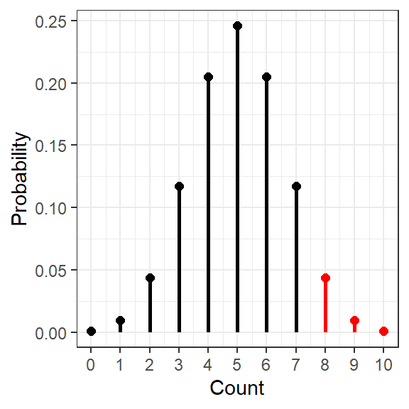

10.1.5 Probability of 80 (or more) out of 100

ex_n = 100
ex_x = 80
ex_p = .50

dbinom(x    = ex_x, 
       size = ex_n, 
       prob = ex_p)

[1] 4.228163e-10

data.frame(count = 0:ex_n) %>% 
  dplyr::mutate(prob = dbinom(count, size = ex_n, p = ex_p)) %>% 
  dplyr::mutate(mark = cut(count, 
                           breaks = c(0, ex_x, ex_n),
                           include.lowest = TRUE)) %>% 
  ggplot(aes(x = count,
             y = prob,
             color = mark)) +
  geom_point() +
  geom_segment(aes(xend = count, 
                   y = 0, 
                   yend = prob)) +
  theme_bw() +
  scale_x_continuous() +
  scale_color_manual(values = c("black", "red")) +
  labs(x = "Count",
       y = "Probability") +
  theme(legend.position = "none")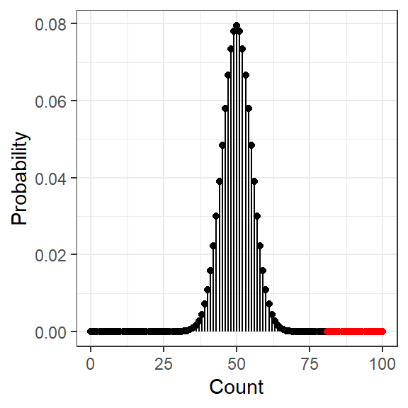

10.2 Example: Fair Coin?

Experiment A coin is flipped ten times and lands on heads eight times

Quesiton Is coin biased?

Hypotheses $$ H_0: Proportion (X) = .50 \

H_1: Proportion (X) .50 $$

10.2.1 Enter tabulated data (subtotals)

tab_coin <- c(heads = 8,
              tails = 2) %>%
  as.table()

tab_coin %>% 
  addmargins()

heads tails   Sum 
    8     2    10 

10.2.2 Two-sided Test

defaults

• Fifty-fifty change: \(H_0: P = .50 \rightarrow\) p = 0.50
• Two-sided alternative: alternative = "two.sided"
• 95% confidence interval: conf.level = 0.95

tab_coin %>%
  binom.test()

    Exact binomial test

data:  .
number of successes = 8, number of trials = 10, p-value = 0.1094
alternative hypothesis: true probability of success is not equal to 0.5
95 percent confidence interval:
 0.4439045 0.9747893
sample estimates:
probability of success 
                   0.8 

10.2.3 One-sided Test

tab_coin %>%
  binom.test(alternative = "greater")

    Exact binomial test

data:  .
number of successes = 8, number of trials = 10, p-value = 0.05469
alternative hypothesis: true probability of success is greater than 0.5
95 percent confidence interval:
 0.4930987 1.0000000
sample estimates:
probability of success 
                   0.8