9 Scatterplots

Using the ggplot2::geom_point() function

library(tidyverse)       # super helpful everything, including ggplot

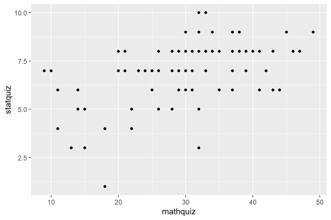
9.1 Two continuous variables

data_ihno %>% 
  ggplot() +
  aes(x = mathquiz,
      y = statquiz) +
  geom_point()

data_ihno %>% 
  dplyr::mutate(phobia_cut3 = cut(phobia, 
                                  breaks = c(0, 2, 4, 10),
                                  include.lowest = TRUE)) %>% 
  ggplot() +
  aes(x = mathquiz,
      y = statquiz,
      color = phobia_cut3) +
  geom_point()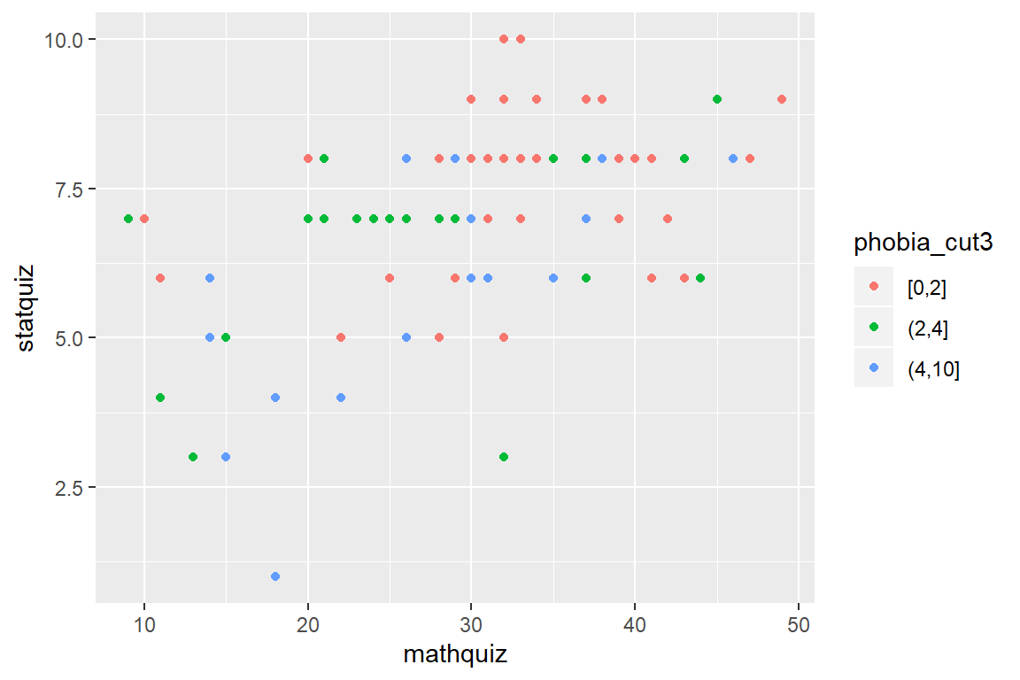

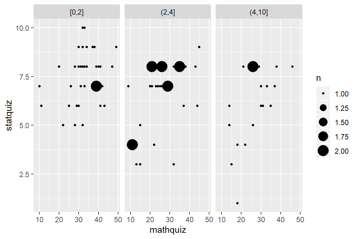
data_ihno %>% 
  dplyr::mutate(phobia_cut3 = cut(phobia, 
                                  breaks = c(0, 2, 4, 10),
                                  include.lowest = TRUE)) %>% 
  ggplot() +
  aes(x = mathquiz,
      y = statquiz) +
  geom_count() +
  facet_grid(. ~ phobia_cut3)