11 1-way Chi Square Test, “Goodness of Fit”

library(tidyverse)
library(effectsize)
library(pander)

11.1 Chi Squared Distribution

data.frame(count = 0:50) %>% 
  dplyr::mutate(prob = dchisq(x = count, df = 1)) %>% 
  ggplot(aes(x = count,
             y = prob)) +
  geom_point() +
  geom_segment(aes(xend = count, 
                   y = 0, 
                   yend = prob),
               size = .1) +
  theme_bw() +
  scale_x_continuous() +
  labs(x = "Count",
       y = "Probability") +
  theme(legend.position = "none")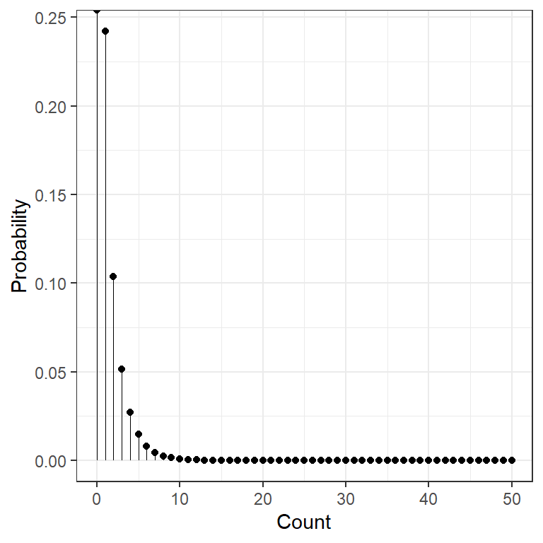

data.frame(count = 0:50) %>% 
  dplyr::mutate(prob = dchisq(x = count, df = 5)) %>% 
  ggplot(aes(x = count,
             y = prob)) +
  geom_point() +
  geom_segment(aes(xend = count, 
                   y = 0, 
                   yend = prob),
               size = .1) +
  theme_bw() +
  scale_x_continuous() +
  labs(x = "Count",
       y = "Probability") +
  theme(legend.position = "none")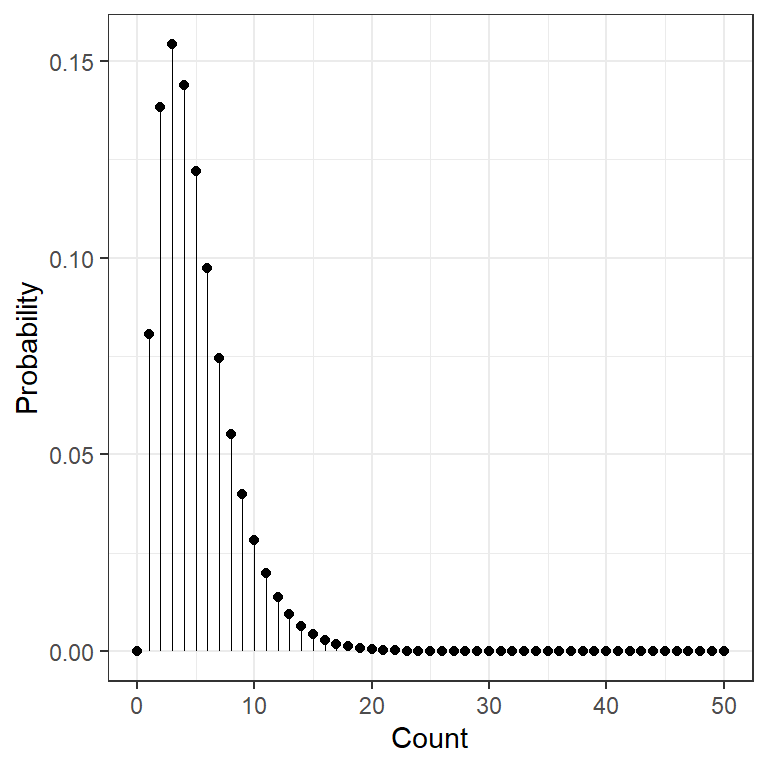

data.frame(count = 0:50) %>% 
  dplyr::mutate(prob = dchisq(x = count, df = 20)) %>% 
  ggplot(aes(x = count,
             y = prob)) +
  geom_point() +
  geom_segment(aes(xend = count, 
                   y = 0, 
                   yend = prob),
               size = .1) +
  theme_bw() +
  scale_x_continuous() +
  labs(x = "Count",
       y = "Probability") +
  theme(legend.position = "none")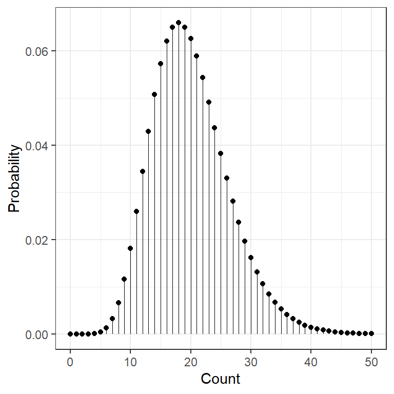

data.frame(count = 0:150) %>% 
  dplyr::mutate(prob = dchisq(x = count, df = 100)) %>% 
  ggplot(aes(x = count,
             y = prob)) +
  geom_point() +
  geom_segment(aes(xend = count, 
                   y = 0, 
                   yend = prob),
               size = .1) +
  theme_bw() +
  scale_x_continuous() +
  labs(x = "Count",
       y = "Probability") +
  theme(legend.position = "none")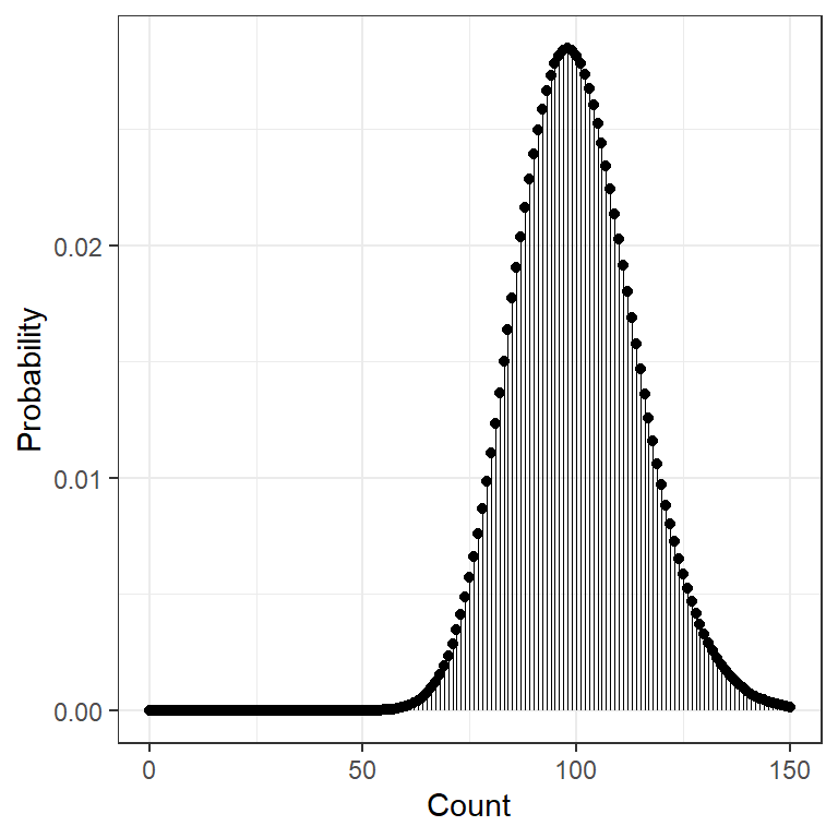

data.frame(count = 0:150) %>% 
  dplyr::mutate(prob_2   = dchisq(x = count, df = 2)) %>% 
  dplyr::mutate(prob_5   = dchisq(x = count, df = 5)) %>% 
  dplyr::mutate(prob_20  = dchisq(x = count, df = 20)) %>% 
  dplyr::mutate(prob_100 = dchisq(x = count, df = 100)) %>% 
  tidyr::pivot_longer(cols = starts_with("prob"),
                      names_to = "df",
                      names_prefix = "prob_",
                      names_ptypes = list(df = factor()),
                      values_to = "prob") %>% 
  dplyr::mutate(mu = df %>% 
                  as.character() %>% 
                  as.numeric()) %>% 
  dplyr::mutate(df = paste0("df = ", df) %>% 
                  factor(levels = c("df = 2",
                                    "df = 5",
                                    "df = 20",
                                    "df = 100"))) %>% 
  ggplot(aes(x = count,
             y = prob)) +
  geom_point(alpha = .4) +
  geom_segment(aes(xend = count, 
                   y = 0, 
                   yend = prob),
               alpha = .4) +
  theme_bw() +
  scale_x_continuous() +
  labs(x = "Count",
       y = "Probability") +
  theme(legend.position = "none") +
  facet_wrap(. ~ df, nrow = 2, scales = "free_y") +
  geom_vline(aes(xintercept = mu),
             color = "red")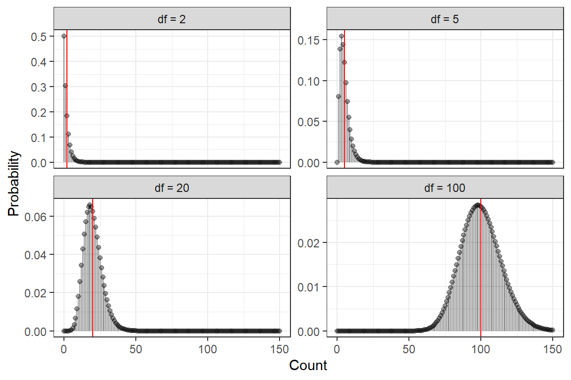

11.2 Chi Squared Test

The chisq.test() function in the base R stats package can be used to perform a Goodnes-of-Fit or one-way Chi-Squared test. This assesses if the observed counts are significantly different from a given profile. The comparison or expected counts may be based on all levels being equally likely or any other specification.

Steps: 1. Enter the data as a ‘concatinated vector’ and change it to the class ‘table’ 2. Perform the test, saving the model fit 3. Extract the observed and expected counts 4. Extract the test output 5. Write up the methods & results

11.3 Null Hypothesis: Equally Likely

Frequently we will to test if there is any difference between the counts in groups. This omnibus test compares the counts in each group to the uniform distribution. This means the expected count in all groups is the same. The expected counts may be found by dividing the total sample by the number of groups.

11.3.1 Ex. Senator Support

A Senator supports a bill favoring stem cell research. However, she realizes her vote could influence whether or not her constituents endorse her bid for re-election. She decides to vote for the bill only if 50% of her constituents support this type of research.

In a random survey of 200 constituents, 96 are in favor of stem cell research. Will the senator support the bill?

tab_vote <- c(support = 96,
              against = 104) %>%
  as.table()

tab_vote %>% 
  addmargins()

support against     Sum 
     96     104     200

Defaults

Null Hypothesis: “equally likely” p = c(1/k, 1/k, 1/k, ... 1/k)

k = number of categories

fit_chisq_vote <- tab_vote %>%
  chisq.test()

fit_chisq_vote$observed

support against 
     96     104

fit_chisq_vote$expected

support against 
    100     100

fit_chisq_vote


    Chi-squared test for given probabilities

data:  .
X-squared = 0.32, df = 1, p-value = 0.5716

11.3.2 Ex. Books

Question:

Is there a difference in number of books checked out for different days of the week?

11.3.2.1 Enter observed counts

This example is given in the Barry Cohen textbook. The library counts the number of books checked out each day for a week. The counts are entered below.

my_book_counts <- c(Monday    = 20,
                    Tuesday   = 14,
                    Wednesday = 18,
                    Thursday  = 17,
                    Friday    = 22,
                    Saturday  = 29) %>% 
  as.table()

my_book_counts

   Monday   Tuesday Wednesday  Thursday    Friday  Saturday 
       20        14        18        17        22        29

11.3.2.2 Perform the test, saving the model fit

NOTE: You do not need to declare any options inside the chisq.test() function, as the default is to use equally likely probabilities.

fit_book_chisq_el <- my_book_counts %>% 
  chisq.test()

11.3.2.3 Extract the observed and expected counts

You can ask for the observed counts. These are just the data your entered into the test.

NOTE: The observed counts MUST be whole numbers!

fit_book_chisq_el$observed

   Monday   Tuesday Wednesday  Thursday    Friday  Saturday 
       20        14        18        17        22        29

You can also ask for the expected counts. The default is for each group to have the total sample divided equally.

NOTE: The expected counts CAN be decimal values.

fit_book_chisq_el$expected

   Monday   Tuesday Wednesday  Thursday    Friday  Saturday 
       20        20        20        20        20        20

You can use the code below to create a single table with both the observed and expected counts, as well as the total for each.

rbind(Observed = fit_book_chisq_el$observed,
      Expected = fit_book_chisq_el$expected,
      Residual = fit_book_chisq_el$observed - fit_book_chisq_el$expected) %>% 
  as.table() %>% 
  addmargins(margin = 2) %>% 
  pander::pander()

	Monday	Tuesday	Wednesday	Thursday	Friday	Saturday	Sum
Observed	20	14	18	17	22	29	120
Expected	20	20	20	20	20	20	120
Residual	0	-6	-2	-3	2	9	0

11.3.2.4 Extract the test output

fit_book_chisq_el


    Chi-squared test for given probabilities

data:  .
X-squared = 6.7, df = 5, p-value = 0.2439

11.3.2.5 Visualize

my_book_counts %>% 
  data.frame() %>% 
  ggplot(aes(x = Var1,
             y = Freq)) +
  geom_col(alpha = .4,
           color = "black") +
  geom_hline(yintercept = 20,
             color = "red",
             size = 2) +
  theme_bw() +
  labs(x = NULL,
       y = "Observed Count")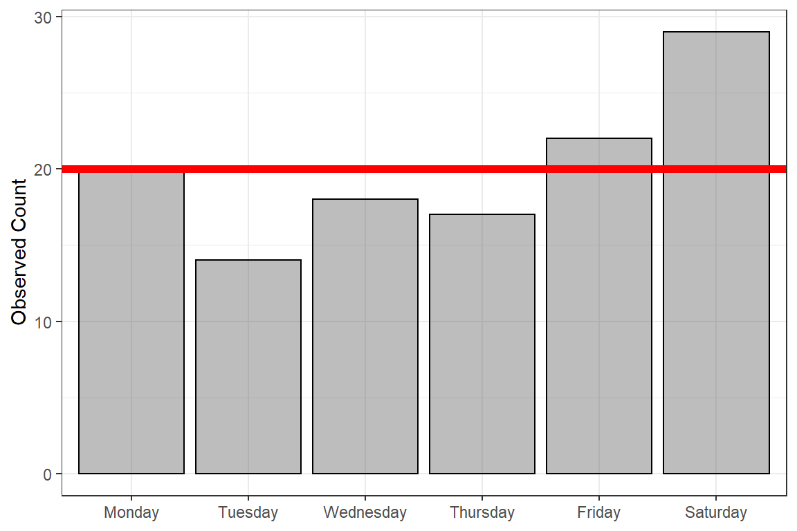

11.3.2.6 Write-up

Methods

To assess if books are checked out uniformly throughout the week, a 1-way Chi Squared Goodness of Fit test was conducted.

Results

This one week provides no evidence that books are checked out more or less on any given day, \(\chi^2 (5) = 6.70\), \(p = .244\).

11.3.3 Ex. M & M Colors

11.3.3.1 Enter observed counts

tab_color_counts <- c(brown  = 4,
                     yellow = 2,
                     red    = 10,
                     green  = 23,
                     blue   = 14,
                     orange = 12) %>% 
  as.table()

tab_color_counts

 brown yellow    red  green   blue orange 
     4      2     10     23     14     12

11.3.3.2 Perform the test, saving the model fit

NOTE: You do not need to declare any options inside the chisq.test() function, as the default is to use equally likely probabilities.

fit_chisq_el <- tab_color_counts %>% 
  chisq.test()

11.3.3.3 Extract the observed and expected counts

You can ask for the observed counts. These are just the data your entered into the test.

NOTE: The observed counts MUST be whole numbers!

fit_chisq_el$observed

 brown yellow    red  green   blue orange 
     4      2     10     23     14     12

You can also ask for the expected counts. The default is for each group to have the total sample divided equally.

NOTE: The expected counts CAN be decimal values.

fit_chisq_el$expected

   brown   yellow      red    green     blue   orange 
10.83333 10.83333 10.83333 10.83333 10.83333 10.83333

You can use the code below to create a single table with both the observed and expected counts, as well as the total for each.

rbind(Observed = fit_chisq_el$observed,
      Expected = fit_chisq_el$expected,
      Residual = fit_chisq_el$observed - fit_chisq_el$expected) %>% 
  as.table() %>% 
  addmargins(margin = 2) %>% 
  pander::pander()

	brown	yellow	red	green	blue	orange	Sum
Observed	4	2	10	23	14	12	65
Expected	10.83	10.83	10.83	10.83	10.83	10.83	65
Residual	-6.833	-8.833	-0.8333	12.17	3.167	1.167	7.105e-15

11.3.3.4 Extract the test output

fit_chisq_el


    Chi-squared test for given probabilities

data:  .
X-squared = 26.292, df = 5, p-value = 7.831e-05

11.3.3.5 Write-up

Methods

To assess if my bag of M & M’s supports the hypothesis that all colors are equally produced, a 1-way Chi Squared Goodness of Fit test was conducted.

Results

Statistically significant evidence was found that not all the colors are equally produced, \(\chi^2 (5) = 26.29\), \(p < .001\). There were fewer brown and yellow, as well as more green, than would be expected.

11.4 Null Hypothesis: a Specific Distribution

11.4.1 Ex. M & M Colors

Years ago, the Mars company used to post the ‘color breakdown’ for each type of M & M it produced on its website. The information has since been removed, but the last time I checked it claim that plain, milk chocolate M & M’s consisted of:

13% brown
14% yellow
13% red
16% green
24% blue
20% orange

11.4.1.1 Perform the test, saving the model fit

NOTE: You DO need to declare any options inside the chisq.test() function, as the default is to use equally likely probabilities.

To compare observed counts to a specified distribution, you need to add that breakdown of 100% (or probability of 1.0) inside the chisq.test(). Make sure that your probabilities add up to EXACTLY ONE! If ther are off by even .00001, it will not run and give and error instead.

fit_chisq_hist <- tab_color_counts %>% 
  chisq.test(p = c(.13, .14, .13, .16, .24, .20))

11.4.1.2 Extract the observed and expected counts

You can use the code below to create a single table with both the observed and expected counts, as well as the total for each.

rbind(Observed = fit_chisq_hist$observed,
      Expected = fit_chisq_hist$expected,
      Residual = fit_chisq_hist$observed - fit_chisq_hist$expected) %>% 
  as.table() %>% 
  addmargins(margin = 2) %>% 
  pander::pander()

	brown	yellow	red	green	blue	orange	Sum
Observed	4	2	10	23	14	12	65
Expected	8.45	9.1	8.45	10.4	15.6	13	65
Residual	-4.45	-7.1	1.55	12.6	-1.6	-1	-3.553e-15

11.4.1.3 Extract the test output

fit_chisq_hist


    Chi-squared test for given probabilities

data:  .
X-squared = 23.674, df = 5, p-value = 0.0002508

11.4.1.4 Write-up

Methods

To assess if my bag of M & M’s supports the reported color breakdown that used to be listed on teh Mars website, a 1-way Chi Squared Goodness of Fit test was conducted.

Results

Statistically significant evidence was found that the color breakdown has changed since the website posting, \(\chi^2 (5) = 23.67\), \(p < .001\). There were fewer brown and yellow, as well as more green, than would be expected if it were still the same.