16 GEE, Binary Outcome: Respiratory Illness
16.1 Packages
16.1.1 CRAN
library(tidyverse)    # all things tidy
library(pander)       # nice looking genderal tabulations
library(furniture)    # nice table1() descriptives
library(texreg)       # Convert Regression Output to LaTeX or HTML Tables
library(psych)        # contains some useful functions, like headTail

library(interactions)
library(performance)
library(lme4)         # Linear, generalized linear, & nonlinear mixed models

library(corrplot)     # Vizualize correlation matrix
library(gee)          # Genderalized Estimation Equation Solver
library(geepack)      # Genderalized Estimation Equation Package
library(MuMIn)        # Multi-Model Inference (caluclate QIC)

library(HSAUR) # package with the dataset16.2 Background
This dataset was used as an example in Chapter 11 of “A Handbook of Statistical Analysis using R” by Brian S. Everitt and Torsten Hothorn. The authors include this data set in their HSAUR package on
CRAN.
The Background
In each of two centers, eligible patients were randomly assigned to active treatment or placebo. During the treatment, the respiratory status (categorized poor or good) was determined at each of four, monthly visits. The trial recruited 111 participants (54 in the active group, 57 in the placebo group) and there were no missing data for either the responses or the covariates.
The Research Question
The question of interest is to assess whether the treatment is effective and to estimate its effect.
Note: We are NOT interested in change over time, but rather mean differences in the treatment group compared to the placebo group, net of any potential confounding due to age, sex, and site.
The Data
Note that the data (555 observations on the following 7 variables) are in long form, i.e, repeated measurements are stored as additional rows in the data frame.
Indicators
subjectthe patient ID, a factor with levels 1 to 111centrethe study center, a factor with levels 1 and 2
monththe month, each patient was examined at months 0, 1, 2, 3 and 4
Outcome or dependent variable
statusthe respiratory status (response variable), a factor with levels poor and good
Main predictor or independent variable of interest
treatmentthe treatment arm, a factor with levels placebo and treatment
Time-invariant Covariates to control for
sexa factor with levels female and male
agethe age of the patient
16.2.1 Read in the data
data("respiratory", package = "HSAUR")

str(respiratory)
'data.frame': 555 obs. of 7 variables:
$ centre : Factor w/ 2 levels "1","2": 1 1 1 1 1 1 1 1 1 1 ...
$ treatment: Factor w/ 2 levels "placebo","treatment": 1 1 1 1 1 1 1 1 1 1 ...
$ sex : Factor w/ 2 levels "female","male": 1 1 1 1 1 1 1 1 1 1 ...
$ age : num 46 46 46 46 46 28 28 28 28 28 ...
$ status : Factor w/ 2 levels "poor","good": 1 1 1 1 1 1 1 1 1 1 ...
$ month : Ord.factor w/ 5 levels "0"<"1"<"2"<"3"<..: 1 2 3 4 5 1 2 3 4 5 ...
$ subject : Factor w/ 111 levels "1","2","3","4",..: 1 1 1 1 1 2 2 2 2 2 ...psych::headTail(respiratory) centre treatment sex age status month subject
1 1 placebo female 46 poor 0 1
112 1 placebo female 46 poor 1 1
223 1 placebo female 46 poor 2 1
334 1 placebo female 46 poor 3 1
... <NA> <NA> <NA> ... <NA> <NA> <NA>
222 2 treatment female 31 good 1 111
333 2 treatment female 31 good 2 111
444 2 treatment female 31 good 3 111
555 2 treatment female 31 good 4 11116.2.2 Wide Format
Wide format has one line per participant.
data_wide <- respiratory %>%
  tidyr::spread(key = month,
                value = status,
                sep = "_") %>%
  dplyr::rename("BL_status" = "month_0") %>%
  dplyr::arrange(subject) %>%
  dplyr::select(subject, centre,
                sex, age, treatment,
                BL_status, starts_with("month"))

tibble::glimpse(data_wide)
Rows: 111
Columns: 10
$ subject <fct> 1, 2, 3, 4, 5, 6, 7, 8, 9, 10, 11, 12, 13, 14, 15, 16, 17, 1…
$ centre <fct> 1, 1, 1, 1, 1, 1, 1, 1, 1, 1, 1, 1, 1, 1, 1, 1, 1, 1, 1, 1, …
$ sex <fct> female, female, female, female, male, female, female, female…
$ age <dbl> 46, 28, 23, 44, 13, 34, 43, 28, 31, 37, 30, 14, 23, 30, 20, …
$ treatment <fct> placebo, placebo, treatment, placebo, placebo, treatment, pl…
$ BL_status <fct> poor, poor, good, good, good, poor, poor, poor, good, good, …
$ month_1 <fct> poor, poor, good, good, good, poor, good, poor, good, poor, …
$ month_2 <fct> poor, poor, good, good, good, poor, poor, poor, good, good, …
$ month_3 <fct> poor, poor, good, good, good, poor, good, poor, good, good, …
$ month_4 <fct> poor, poor, good, poor, good, poor, good, poor, good, poor, …psych::headTail(data_wide) subject centre sex age treatment BL_status month_1 month_2 month_3
1 1 1 female 46 placebo poor poor poor poor
2 2 1 female 28 placebo poor poor poor poor
3 3 1 female 23 treatment good good good good
4 4 1 female 44 placebo good good good good
... <NA> <NA> <NA> ... <NA> <NA> <NA> <NA> <NA>
108 108 2 male 39 treatment poor good good good
109 109 2 female 68 treatment poor good good good
110 110 2 male 63 treatment good good good good
111 111 2 female 31 treatment good good good good
month_4
1 poor
2 poor
3 good
4 poor
... <NA>
108 good
109 good
110 good
111 good16.2.3 Long Format
Long format has one line per observation.
data_long <- data_wide%>%
  tidyr::gather(key = month,
                value = status,
                starts_with("month")) %>%
  dplyr::mutate(month = str_sub(month, start = -1) %>% as.numeric) %>%
  dplyr::mutate(status = case_when(status == "poor" ~ 0,
                                   status == "good" ~ 1)) %>%
  dplyr::arrange(subject, month) %>%
  dplyr::select(subject, centre, sex, age, treatment, BL_status, month, status)


tibble::glimpse(data_long)
Rows: 444
Columns: 8
$ subject <fct> 1, 1, 1, 1, 2, 2, 2, 2, 3, 3, 3, 3, 4, 4, 4, 4, 5, 5, 5, 5, …
$ centre <fct> 1, 1, 1, 1, 1, 1, 1, 1, 1, 1, 1, 1, 1, 1, 1, 1, 1, 1, 1, 1, …
$ sex <fct> female, female, female, female, female, female, female, fema…
$ age <dbl> 46, 46, 46, 46, 28, 28, 28, 28, 23, 23, 23, 23, 44, 44, 44, …
$ treatment <fct> placebo, placebo, placebo, placebo, placebo, placebo, placeb…
$ BL_status <fct> poor, poor, poor, poor, poor, poor, poor, poor, good, good, …
$ month <dbl> 1, 2, 3, 4, 1, 2, 3, 4, 1, 2, 3, 4, 1, 2, 3, 4, 1, 2, 3, 4, …
$ status <dbl> 0, 0, 0, 0, 0, 0, 0, 0, 1, 1, 1, 1, 1, 1, 1, 0, 1, 1, 1, 1, …psych::headTail(data_long) subject centre sex age treatment BL_status month status
1 1 1 female 46 placebo poor 1 0
2 1 1 female 46 placebo poor 2 0
3 1 1 female 46 placebo poor 3 0
4 1 1 female 46 placebo poor 4 0
... <NA> <NA> <NA> ... <NA> <NA> ... ...
441 111 2 female 31 treatment good 1 1
442 111 2 female 31 treatment good 2 1
443 111 2 female 31 treatment good 3 1
444 111 2 female 31 treatment good 4 116.3 Exploratory Data Analysis
16.3.1 Summary Statistics
16.3.1.1 Demographics and Baseline Measure
Notice that numerical summaries are computed for all variables, even the categorical variables (i.e. factors). The have an * after the variable name to remind you that the mean, sd, and se are of limited use.
Notice: the mean age is 33
data_wide %>%
  psych::describe(skew = FALSE)
vars n mean sd min max range se
subject* 1 111 56.00 32.19 1 111 110 3.06
centre* 2 111 1.50 0.50 1 2 1 0.05
sex* 3 111 1.21 0.41 1 2 1 0.04
age 4 111 33.28 13.65 11 68 57 1.30
treatment* 5 111 1.49 0.50 1 2 1 0.05
BL_status* 6 111 1.45 0.50 1 2 1 0.05
month_1* 7 111 1.59 0.49 1 2 1 0.05
month_2* 8 111 1.54 0.50 1 2 1 0.05
month_3* 9 111 1.59 0.49 1 2 1 0.05
month_4* 10 111 1.53 0.50 1 2 1 0.05data_wide %>%
dplyr::group_by(treatment) %>%
furniture::table1("Center" = centre,
"Sex" = sex,
"Age" = age,
"Baseline Status" = BL_status,
caption = "Participant Demographics",
output = "markdown",
na.rm = FALSE,
total = TRUE,
test = TRUE)| Total | placebo | treatment | P-Value | |
|---|---|---|---|---|
| n = 111 | n = 57 | n = 54 | ||
| Center | 1 | |||
| 1 | 56 (50.5%) | 29 (50.9%) | 27 (50%) | |
| 2 | 55 (49.5%) | 28 (49.1%) | 27 (50%) | |
| NA | 0 (0%) | 0 (0%) | 0 (0%) | |
| Sex | 0.028 | |||
| female | 88 (79.3%) | 40 (70.2%) | 48 (88.9%) | |
| male | 23 (20.7%) | 17 (29.8%) | 6 (11.1%) | |
| NA | 0 (0%) | 0 (0%) | 0 (0%) | |
| Age | 0.771 | |||
| 33.3 (13.7) | 33.6 (13.4) | 32.9 (14.0) | ||
| Baseline Status | 1 | |||
| poor | 61 (55%) | 31 (54.4%) | 30 (55.6%) | |
| good | 50 (45%) | 26 (45.6%) | 24 (44.4%) | |
| NA | 0 (0%) | 0 (0%) | 0 (0%) |
16.3.1.2 Status Over Time
data_wide %>%
  dplyr::group_by(treatment) %>%
  furniture::table1("Month One" = month_1,
                    "Month Two" = month_2,
                    "Month Three" = month_3,
                    "Month Four" = month_4,
                    caption = "Respiratory Status Over Time",
                    output = "markdown",
                    na.rm = FALSE,
                    total = TRUE,
test = TRUE)| Total | placebo | treatment | P-Value | |
|---|---|---|---|---|
| n = 111 | n = 57 | n = 54 | ||
| Month One | 0.06 | |||
| poor | 46 (41.4%) | 29 (50.9%) | 17 (31.5%) | |
| good | 65 (58.6%) | 28 (49.1%) | 37 (68.5%) | |
| NA | 0 (0%) | 0 (0%) | 0 (0%) | |
| Month Two | 0.002 | |||
| poor | 51 (45.9%) | 35 (61.4%) | 16 (29.6%) | |
| good | 60 (54.1%) | 22 (38.6%) | 38 (70.4%) | |
| NA | 0 (0%) | 0 (0%) | 0 (0%) | |
| Month Three | 0.008 | |||
| poor | 46 (41.4%) | 31 (54.4%) | 15 (27.8%) | |
| good | 65 (58.6%) | 26 (45.6%) | 39 (72.2%) | |
| NA | 0 (0%) | 0 (0%) | 0 (0%) | |
| Month Four | 0.068 | |||
| poor | 52 (46.8%) | 32 (56.1%) | 20 (37%) | |
| good | 59 (53.2%) | 25 (43.9%) | 34 (63%) | |
| NA | 0 (0%) | 0 (0%) | 0 (0%) |
Correlation between repeated observations:
data_wide %>%
  dplyr::select(starts_with("month")) %>%
  dplyr::mutate_all(function(x) x == "good") %>%
  cor() %>%
  corrplot::corrplot.mixed()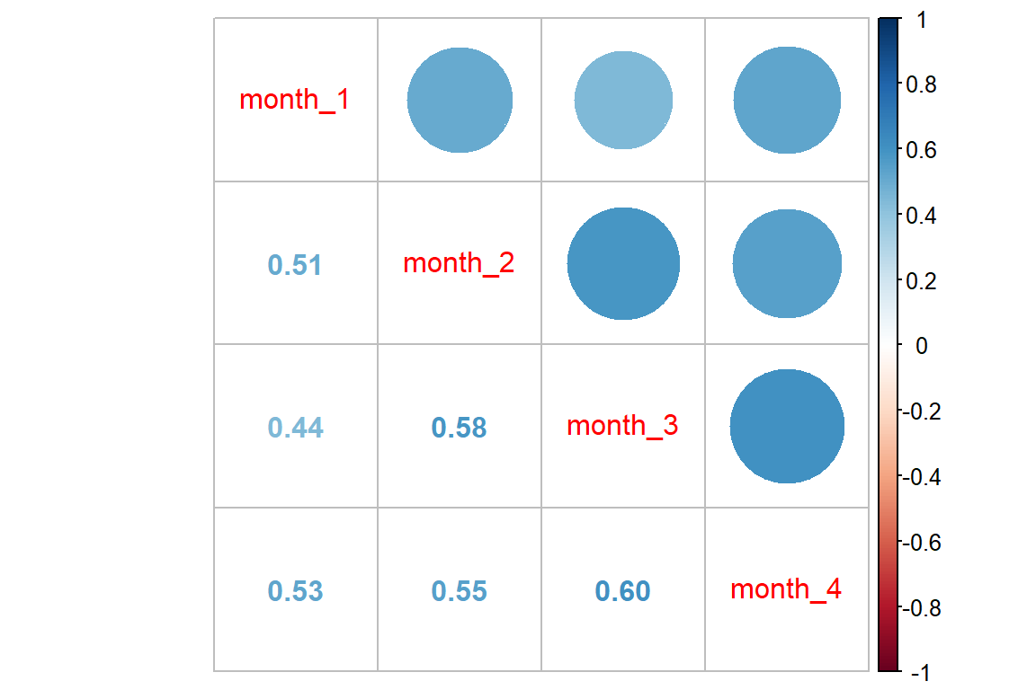
data_month_trt_prop <- data_long %>%
  dplyr::group_by(treatment, month) %>%
  dplyr::summarise(n = n(),
                   prop_good = mean(status),
                   prop_sd = sd(status),
                   prop_se = prop_sd/sqrt(n))

data_month_trt_prop
# A tibble: 8 × 6
# Groups: treatment [2]
treatment month n prop_good prop_sd prop_se
<fct> <dbl> <int> <dbl> <dbl> <dbl>
1 placebo 1 57 0.491 0.504 0.0668
2 placebo 2 57 0.386 0.491 0.0651
3 placebo 3 57 0.456 0.503 0.0666
4 placebo 4 57 0.439 0.501 0.0663
5 treatment 1 54 0.685 0.469 0.0638
6 treatment 2 54 0.704 0.461 0.0627
7 treatment 3 54 0.722 0.452 0.0615
8 treatment 4 54 0.630 0.487 0.066316.3.2 Visualization
16.3.2.1 Age
data_wide %>%
  ggplot(aes(age)) +
  geom_histogram(binwidth = 5,
                 color = "black",
                 alpha = .3) +
  geom_vline(xintercept = c(20, 35, 45),
             color = "red") +
  theme_bw() +
  facet_grid(treatment ~ .)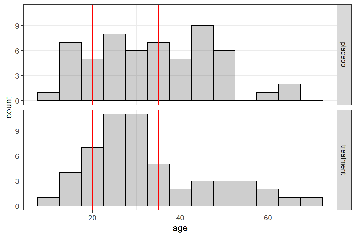
16.3.2.2 Status by Age
data_wide %>%
  dplyr::mutate(n_good = furniture::rowsums(month_1 == "good",
                                            month_2 == "good",
                                            month_3 == "good",
                                            month_4 == "good")) %>%
  ggplot(aes(x = age,
             y = n_good)) +
  geom_count() +
  geom_smooth() +
  theme_bw() +
  labs(x = "Age in Years",
       y = "Number of Visits out of Four, with 'Good' Respiration")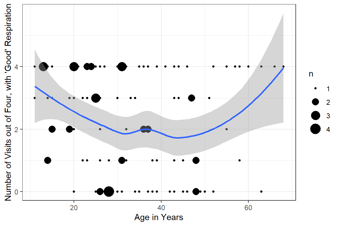
16.3.2.3 Status Over Time
It apears that status is fairly constant over time.
data_month_trt_prop %>%
  ggplot(aes(x = month,
             y = prop_good,
             group = treatment,
             color = treatment)) +
  geom_errorbar(aes(ymin = prop_good - prop_se,
                    ymax = prop_good + prop_se),
                width = .25) +
  geom_point() +
  geom_line() +
  theme_bw() +
  labs(x = "Time, months",
       y = "Proportion of Participants\nwith 'Good' Respiratory Status") +
  theme(legend.position = "bottom",
        legend.key.width = unit(1.5, "cm"))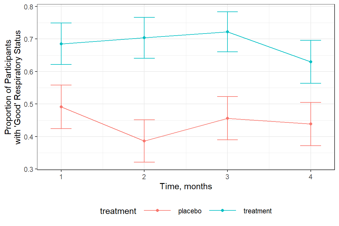
It is NOT the purpose of this analysis to investigate change over time!
Since status is largely stable over time, no linear (or even
quadratic) effect of the month variable will be
modeled.
Instead, the four observations on each subject are treated as correlated (at least with non-independent correlation structure in GEE), but no time trend will be included.
16.4 Logisitc Regression (GLM)
Note: THIS IS NEVER APPROPRIATE TO CONDUCT A GLM ON REPEATED MEASURES. THIS IS DONE FOR ILLUSTRATION PURPOSES ONLY!
Since participants in the middle ages seem to do worse than either extreme, the potential quadratic effect of age will be included. Age is also being grand-mean centered to make the intercept more meaningful.
16.4.1 Fit the Model
resp_glm <- glm(status ~ centre + treatment + sex + BL_status +
                  I(age-33) + I((age-33)^2),
                data = data_long,
                family = binomial(link = "logit"))

summary(resp_glm)
Call:
glm(formula = status ~ centre + treatment + sex + BL_status +
    I(age - 33) + I((age - 33)^2), family = binomial(link = "logit"),
    data = data_long)

Deviance Residuals:
    Min       1Q   Median       3Q      Max
-2.5965  -0.9178   0.3985   0.8388   2.0988

Coefficients:
                     Estimate Std. Error z value Pr(>|z|)
(Intercept)        -1.9685725  0.2733549  -7.202 5.95e-13 ***
centre2             0.5347938  0.2464412   2.170 0.030002 *
treatmenttreatment  1.3561814  0.2447533   5.541 3.01e-08 ***
sexmale             0.4263433  0.3175081   1.343 0.179343
BL_statusgood       1.9193401  0.2500033   7.677 1.63e-14 ***
I(age - 33)        -0.0368535  0.0106382  -3.464 0.000532 ***
I((age - 33)^2)     0.0025169  0.0006352   3.963 7.41e-05 ***
---
Signif. codes:  0 '***' 0.001 '**' 0.01 '*' 0.05 '.' 0.1 ' ' 1

(Dispersion parameter for binomial family taken to be 1)

    Null deviance: 608.93  on 443  degrees of freedom
Residual deviance: 465.25  on 437  degrees of freedom
AIC: 479.25

Number of Fisher Scoring iterations: 4
16.4.2 Tabulate the Model Parameters
texreg::knitreg(list(resp_glm,
                     texreghelpr::extract_glm_exp(resp_glm,
                                                  include.any = FALSE)),
                custom.model.names = c("b (SE)", "OR [95 CI]"),
                caption = "Logistic Generalized Linear Regression (GLM)",
                single.row = TRUE,
                digits = 3,
ci.test = 1)| b (SE) | OR [95 CI] | |
|---|---|---|
| (Intercept) | -1.969 (0.273)*** | 0.140 [0.080; 0.234]* |
| centre2 | 0.535 (0.246)* | 1.707 [1.054; 2.775]* |
| treatmenttreatment | 1.356 (0.245)*** | 3.881 [2.422; 6.334]* |
| sexmale | 0.426 (0.318) | 1.532 [0.826; 2.875] |
| BL_statusgood | 1.919 (0.250)*** | 6.816 [4.221; 11.271]* |
| age - 33 | -0.037 (0.011)*** | 0.964 [0.943; 0.984]* |
| (age - 33)^2 | 0.003 (0.001)*** | 1.003 [1.001; 1.004]* |
| AIC | 479.253 | |
| BIC | 507.924 | |
| Log Likelihood | -232.626 | |
| Deviance | 465.253 | |
| Num. obs. | 444 | |
| ***p < 0.001; **p < 0.01; *p < 0.05 (or Null hypothesis value outside the confidence interval). | ||
16.5 Generalized Estimating Equations (GEE)
Again, since participants age is likely to be a risk at either end of the spectrum, the potential quadratic effect of age will be modeled. Age is also being grand-mean centered to make the intercept more meaningful.
16.5.1 Indepdendence
Using an "independence" correlation structure is equivalent to using a GLM analysis (logistic regression in this case) and is never appropriate for repeated measures data. It is only being done here for comparison purposes.
resp_gee_in <- gee::gee(status ~ centre + treatment + sex + BL_status +
                          I(age-33) + I((age-33)^2),
                        data = data_long,
                        family = binomial(link = "logit"),
                        id = subject,
                        corstr = "independence",
                        scale.fix = TRUE,
                        scale.value = 1)
(Intercept) centre2 treatmenttreatment sexmale
-1.968572485 0.534793799 1.356181372 0.426343291
BL_statusgood I(age - 33) I((age - 33)^2)
1.919340141 -0.036853528 0.002516859 summary(resp_gee_in)
 GEE:  GENERALIZED LINEAR MODELS FOR DEPENDENT DATA
 gee S-function, version 4.13 modified 98/01/27 (1998)

Model:
 Link:                      Logit
 Variance to Mean Relation: Binomial
 Correlation Structure:     Independent

Call:
gee::gee(formula = status ~ centre + treatment + sex + BL_status +
    I(age - 33) + I((age - 33)^2), id = subject, data = data_long,
    family = binomial(link = "logit"), corstr = "independence",
    scale.fix = TRUE, scale.value = 1)

Summary of Residuals:
        Min          1Q      Median          3Q         Max
-0.96563962 -0.34372730  0.07631922  0.29658264  0.88947816


Coefficients:
                       Estimate   Naive S.E.   Naive z  Robust S.E.   Robust z
(Intercept)        -1.968572493 0.2733635751 -7.201298 0.4457014141 -4.4167966
centre2             0.534793799 0.2464443046  2.170039 0.3795759846  1.4089242
treatmenttreatment  1.356181377 0.2447584751  5.540896 0.3777998909  3.5896818
sexmale             0.426343293 0.3175134753  1.342757 0.4832336627  0.8822715
BL_statusgood       1.919340146 0.2500092510  7.677077 0.3772812271  5.0872930
I(age - 33)        -0.036853528 0.0106384086 -3.464196 0.0150120266 -2.4549336
I((age - 33)^2)     0.002516859 0.0006351834  3.962414 0.0007592432  3.3149582

Estimated Scale Parameter:  1
Number of Iterations:  1

Working Correlation
     [,1] [,2] [,3] [,4]
[1,]    1    0    0    0
[2,]    0    1    0    0
[3,]    0    0    1    0
[4,]    0    0    0    1
The results for GEE fit with the independence correlation structure produces results that are nearly identical to the GLM model.
The robust (sandwich) standard errors are however much larger than the naive standard errors.
16.5.2 Exchangeable
resp_gee_ex <- gee::gee(status ~ centre + treatment + sex + BL_status +
                          I(age-33) + I((age-33)^2),
                        data = data_long,
                        family = binomial(link = "logit"),
                        id = subject,
                        corstr = "exchangeable",
                        scale.fix = TRUE,
                        scale.value = 1)
(Intercept) centre2 treatmenttreatment sexmale
-1.968572485 0.534793799 1.356181372 0.426343291
BL_statusgood I(age - 33) I((age - 33)^2)
1.919340141 -0.036853528 0.002516859 summary(resp_gee_ex)
 GEE:  GENERALIZED LINEAR MODELS FOR DEPENDENT DATA
 gee S-function, version 4.13 modified 98/01/27 (1998)

Model:
 Link:                      Logit
 Variance to Mean Relation: Binomial
 Correlation Structure:     Exchangeable

Call:
gee::gee(formula = status ~ centre + treatment + sex + BL_status +
    I(age - 33) + I((age - 33)^2), id = subject, data = data_long,
    family = binomial(link = "logit"), corstr = "exchangeable",
    scale.fix = TRUE, scale.value = 1)

Summary of Residuals:
        Min          1Q      Median          3Q         Max
-0.96563962 -0.34372730  0.07631922  0.29658264  0.88947816


Coefficients:
                       Estimate  Naive S.E.    Naive z  Robust S.E.   Robust z
(Intercept)        -1.968572493 0.379830796 -5.1827617 0.4457014141 -4.4167966
centre2             0.534793799 0.342427246  1.5617735 0.3795759846  1.4089242
treatmenttreatment  1.356181377 0.340084835  3.9877737 0.3777998909  3.5896818
sexmale             0.426343293 0.441175807  0.9663796 0.4832336627  0.8822715
BL_statusgood       1.919340146 0.347380636  5.5251789 0.3772812271  5.0872930
I(age - 33)        -0.036853528 0.014781762 -2.4931757 0.0150120266 -2.4549336
I((age - 33)^2)     0.002516859 0.000882569  2.8517424 0.0007592432  3.3149582

Estimated Scale Parameter:  1
Number of Iterations:  1

Working Correlation
        [,1]    [,2]    [,3]    [,4]
[1,] 1.00000 0.31021 0.31021 0.31021
[2,] 0.31021 1.00000 0.31021 0.31021
[3,] 0.31021 0.31021 1.00000 0.31021
[4,] 0.31021 0.31021 0.31021 1.00000
Notice that the naive standard errors are more similar to the robust (sandwich) standard errors, supporting that this is a better fitting model
16.5.3 Paramgeter Estimates Table
The GEE models display the robust (sandwich) standard errors.
16.5.3.1 Raw Estimates (Logit Scale)
texreg::knitreg(list(resp_glm,
                     resp_gee_in,
                     resp_gee_ex),
                custom.model.names = c("GLM",
                                       "GEE-INDEP",
                                       "GEE-EXCH"),
                caption = "Estimates on Logit Scale",
                single.row = TRUE,
digits = 4)| GLM | GEE-INDEP | GEE-EXCH | |
|---|---|---|---|
| (Intercept) | -1.9686 (0.2734)*** | -1.9686 (0.4457)*** | -1.9686 (0.4457)*** |
| centre2 | 0.5348 (0.2464)* | 0.5348 (0.3796) | 0.5348 (0.3796) |
| treatmenttreatment | 1.3562 (0.2448)*** | 1.3562 (0.3778)*** | 1.3562 (0.3778)*** |
| sexmale | 0.4263 (0.3175) | 0.4263 (0.4832) | 0.4263 (0.4832) |
| BL_statusgood | 1.9193 (0.2500)*** | 1.9193 (0.3773)*** | 1.9193 (0.3773)*** |
| age - 33 | -0.0369 (0.0106)*** | -0.0369 (0.0150)* | -0.0369 (0.0150)* |
| (age - 33)^2 | 0.0025 (0.0006)*** | 0.0025 (0.0008)*** | 0.0025 (0.0008)*** |
| AIC | 479.2530 | ||
| BIC | 507.9238 | ||
| Log Likelihood | -232.6265 | ||
| Deviance | 465.2530 | ||
| Num. obs. | 444 | 444 | 444 |
| Scale | 1.0000 | 1.0000 | |
| ***p < 0.001; **p < 0.01; *p < 0.05 | |||
Comparing the two GEE models: parameters are identical and so are the robust (sandwich) standard errors.
16.5.3.2 Exponentiate the Estimates (odds ratio scale)
texreg::knitreg(list(extract_glm_exp(resp_glm),
                     extract_gee_exp(resp_gee_in),
                     extract_gee_exp(resp_gee_ex)),
                custom.model.names = c("GLM",
                                       "GEE-INDEP",
                                       "GEE-EXCH"),
                caption = "Estimates on Odds-Ratio Scale",
                single.row = TRUE,
                ci.test = 1,
digits = 3)| GLM | GEE-INDEP | GEE-EXCH | |
|---|---|---|---|
| (Intercept) | 0.140 [0.080; 0.234]* | 0.140 [0.058; 0.335]* | 0.140 [0.058; 0.335]* |
| centre2 | 1.707 [1.054; 2.775]* | 1.707 [0.811; 3.592] | 1.707 [0.811; 3.592] |
| treatmenttreatment | 3.881 [2.422; 6.334]* | 3.881 [1.851; 8.139]* | 3.881 [1.851; 8.139]* |
| sexmale | 1.532 [0.826; 2.875] | 1.532 [0.594; 3.949] | 1.532 [0.594; 3.949] |
| BL_statusgood | 6.816 [4.221; 11.271]* | 6.816 [3.254; 14.279]* | 6.816 [3.254; 14.279]* |
| age - 33 | 0.964 [0.943; 0.984]* | 0.964 [0.936; 0.993]* | 0.964 [0.936; 0.993]* |
| (age - 33)^2 | 1.003 [1.001; 1.004]* | 1.003 [1.001; 1.004]* | 1.003 [1.001; 1.004]* |
| Dispersion | 1.000 | 1.000 | |
| * Null hypothesis value outside the confidence interval. | |||
16.5.3.3 Manual Extraction
resp_gee_ex %>% coef() %>% exp() (Intercept) centre2 treatmenttreatment sexmale
0.1396561 1.7070962 3.8813436 1.5316465
BL_statusgood I(age - 33) I((age - 33)^2)
6.8164591 0.9638173 1.0025200 trt_EST <- summary(resp_gee_ex)$coeff["treatmenttreatment", "Estimate"]
trt_EST[1] 1.356181exp(trt_EST)[1] 3.881344Trt_SE <- summary(resp_gee_ex)$coeff["treatmenttreatment", "Robust S.E."]
Trt_SE[1] 0.3777999trt_95ci <- trt_EST + c(-1, +1)*1.96*Trt_SE
trt_95ci[1] 0.6156936 2.0966692exp(trt_95ci)[1] 1.850940 8.13901516.5.4 Final Model
16.5.4.1 Estimates on both the logit and odds-ratio scales
texreg::knitreg(list(resp_gee_ex,
                     texreghelpr::extract_gee_exp(resp_gee_ex,
                                                  include.any = FALSE)),
                custom.model.names = c("b (SE)",
                                       "OR [95 CI]"),
                custom.coef.map = list("(Intercept)" = "(Intercept)",
                                       centre2 = "Center 2 vs. 1",
                                       sexmale = "Male vs. Female",
                                       BL_statusgood = "BL Good vs. Poor",
                                       "I(age - 33)" = "Age (Yrs post 33)",
                                       "I((age - 33)^2)" = "Age-Squared",
                                       treatmenttreatment = "Treatment"),
                caption = "GEE: Final Model (exchangable)",
                ci.test = 1,
                single.row = TRUE,
digits = 3)| b (SE) | OR [95 CI] | |
|---|---|---|
| (Intercept) | -1.969 (0.446)*** | 0.140 [0.058; 0.335]* |
| Center 2 vs. 1 | 0.535 (0.380) | 1.707 [0.811; 3.592] |
| Male vs. Female | 0.426 (0.483) | 1.532 [0.594; 3.949] |
| BL Good vs. Poor | 1.919 (0.377)*** | 6.816 [3.254; 14.279]* |
| Age (Yrs post 33) | -0.037 (0.015)* | 0.964 [0.936; 0.993]* |
| Age-Squared | 0.003 (0.001)*** | 1.003 [1.001; 1.004]* |
| Treatment | 1.356 (0.378)*** | 3.881 [1.851; 8.139]* |
| Scale | 1.000 | |
| Num. obs. | 444 | |
| Dispersion | 1.000 | |
| ***p < 0.001; **p < 0.01; *p < 0.05 (or Null hypothesis value outside the confidence interval). | ||
16.5.4.2 Interpretation
centre: Controlling for baseline status, sex, age, and treatment, participants at the two centers did not significantly differ in respiratory status during the interventionsex: Controlling for baseline status, center, age, and treatment, a participant’s respiratory status did not differ between the two sexes.BL_status: Controlling for sex, center, age, and treatment, those with good baseline status had nearly 7 times higher odds of having a good respiratory status, compared to participants that starts out poor.age: Controlling for baseline status, sex, center, and treatment, the role of age was non-linear, such that the odds of a good respiratory status was lowest for patients age 40 and better for those that were either younger or older.
Most importantly:
treatment: Controlling for baseline status, sex, age, and center, those on the treatment had 3.88 time higher odds of having a good respiratory status, compared to similar participants that were randomized to the placebo.
16.5.5 Predicted Probabilities
16.5.5.1 Refit with the geepack package
This package lets you plot, but not put the results in a table.
resp_geeglm_ex <- geepack::geeglm(status ~ centre + treatment + sex + BL_status +
                                    I(age-33) + I((age-33)^2),
                                  data = data_long,
                                  family = binomial(link = "logit"),
                                  id = subject,
                                  waves = month,
                                  corstr = "exchangeable")
16.5.5.2 Make predictions
What is the change a 40 year old man in poor condition at center 1 change of being rated as being in “Good” respiratory condition?
resp_geeglm_ex %>%
  emmeans::emmeans(pairwise ~ treatment,
                   at = list(centre = "1",
                             sex = "male",
                             age = 40,
                             BL_status = "poor"),
                   type = "response")
$emmeans
treatment prob SE df asymp.LCL asymp.UCL
placebo 0.158 0.0548 Inf 0.0768 0.296
treatment 0.421 0.1164 Inf 0.2215 0.649
Covariance estimate used: vbeta
Confidence level used: 0.95
Intervals are back-transformed from the logit scale
$contrasts
contrast odds.ratio SE df null z.ratio p.value
placebo / treatment 0.258 0.0973 Inf 1 -3.590 0.0003
Tests are performed on the log odds ratio scale A 40 year old man in poor condition at center 1 has a 15.8% change of being rated as being in “Good” respiratory condition if he was randomized to placebo.
A 40 year old man in poor condition at center 1 has a 42.1% change of being rated as being in “Good” respiratory condition if he was randomized to placebo.
The odds ratio for treatment is:
(.421/(1 -.421) )/( .158/(1 - .158))[1] 3.87488216.5.6 Marginal Plot to Visualize the Model
16.5.6.1 Quickest Version
The interactions::interact_plot() function can only investigate 3 variables at once:
predthe x-axis (must be continuous)modxdifferent lines (may be categorical or continuous)mod2side-by-side panels (may be categorical or continuous)
All other variables must be held constant.
interactions::interact_plot(model = resp_geeglm_ex,   # model name
                            pred = age,               # x-axis
                            modx = treatment,         # lines
                            mod2 = sex,               # panels
                            data = data_long,
                            at = list(centre = "1",
                                      BL_status = "good"),  # hold constant
                            type = "mean_subject") +
  theme_bw()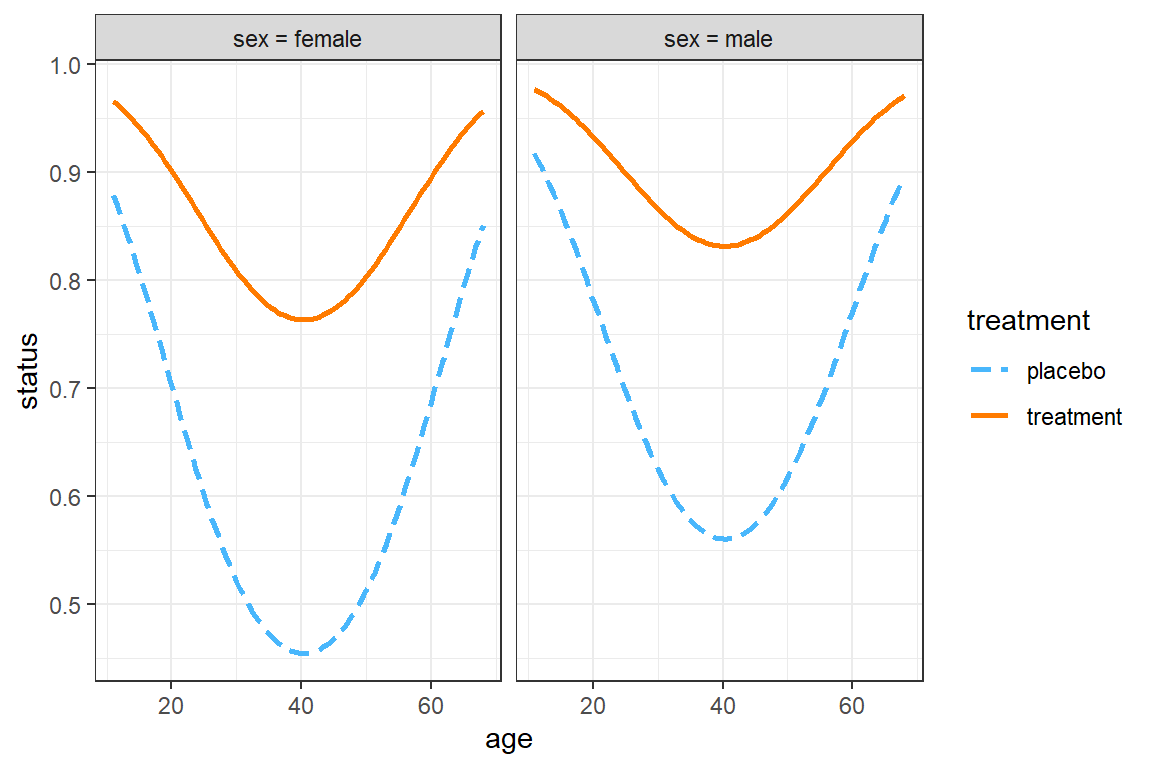
16.5.6.2 Full Version
Makes a dataset with all combinations
resp_geeglm_ex %>%
  emmeans::emmeans(~ centre + treatment + sex + age + BL_status,
                   at = list(age = c(20, 35, 50)),
                   type = "response") %>%
  data.frame()
centre treatment sex age BL_status prob SE df asymp.LCL
1 1 placebo female 20 poor 0.2565215 0.06548740 Inf 0.14967845
2 2 placebo female 20 poor 0.3706723 0.12112814 Inf 0.17551296
3 1 treatment female 20 poor 0.5724989 0.07094442 Inf 0.43141390
4 2 treatment female 20 poor 0.6956880 0.09012479 Inf 0.49811941
5 1 placebo male 20 poor 0.3457476 0.10327449 Inf 0.17761271
6 2 placebo male 20 poor 0.4742752 0.11897826 Inf 0.26149005
7 1 treatment male 20 poor 0.6722540 0.13353316 Inf 0.38474268
8 2 treatment male 20 poor 0.7778518 0.09957372 Inf 0.53090485
9 1 placebo female 35 poor 0.1158621 0.04715858 Inf 0.05047400
10 2 placebo female 35 poor 0.1828109 0.09160156 Inf 0.06302045
11 1 treatment female 35 poor 0.3371478 0.06614826 Inf 0.22163454
12 2 treatment female 35 poor 0.4647493 0.11044788 Inf 0.26669467
13 1 placebo male 35 poor 0.1671630 0.05669685 Inf 0.08286363
14 2 placebo male 35 poor 0.2551987 0.08445543 Inf 0.12543357
15 1 treatment male 35 poor 0.4379004 0.11914059 Inf 0.23176597
16 2 treatment male 35 poor 0.5707977 0.11262714 Inf 0.35070552
17 1 placebo female 50 poor 0.1338069 0.05877875 Inf 0.05408046
18 2 placebo female 50 poor 0.2086774 0.10132831 Inf 0.07340015
19 1 treatment female 50 poor 0.3748352 0.08438493 Inf 0.22840791
20 2 treatment female 50 poor 0.5058160 0.11024112 Inf 0.30129761
21 1 placebo male 50 poor 0.1913338 0.06744244 Inf 0.09148083
22 2 placebo male 50 poor 0.2877016 0.08618754 Inf 0.15047521
23 1 treatment male 50 poor 0.4787165 0.12607341 Inf 0.25438187
24 2 treatment male 50 poor 0.6105461 0.10299001 Inf 0.40147684
25 1 placebo female 20 good 0.7016595 0.07358528 Inf 0.54146521
26 2 placebo female 20 good 0.8005933 0.06259978 Inf 0.65055094
27 1 treatment female 20 good 0.9012681 0.04083868 Inf 0.78782754
28 2 treatment female 20 good 0.9396977 0.02445873 Inf 0.86991509
29 1 placebo male 20 good 0.7827145 0.10216134 Inf 0.52603135
30 2 placebo male 20 good 0.8601276 0.06117585 Inf 0.69417730
31 1 treatment male 20 good 0.9332512 0.04985998 Inf 0.74440141
32 2 treatment male 20 good 0.9597874 0.02684720 Inf 0.85926193
33 1 placebo female 35 good 0.4718119 0.09433741 Inf 0.29842235
34 2 placebo female 35 good 0.6039430 0.10310876 Inf 0.39581143
35 1 treatment female 35 good 0.7761395 0.06499212 Inf 0.62484433
36 2 treatment female 35 good 0.8554625 0.04422313 Inf 0.74594602
37 1 placebo male 35 good 0.5777323 0.12049412 Inf 0.34195766
38 2 placebo male 35 good 0.7002031 0.08237976 Inf 0.51976564
39 1 treatment male 35 good 0.8415295 0.08778590 Inf 0.59374248
40 2 treatment male 35 good 0.9006481 0.04809252 Inf 0.75970156
41 1 placebo female 50 good 0.5129046 0.11084368 Inf 0.30619949
42 2 placebo female 50 good 0.6425442 0.10133622 Inf 0.43086572
43 1 treatment female 50 good 0.8034205 0.06889169 Inf 0.63480235
44 2 treatment female 50 good 0.8746381 0.04007282 Inf 0.77316863
45 1 placebo male 50 good 0.6172692 0.12419998 Inf 0.36530393
46 2 placebo male 50 good 0.7335613 0.07358316 Inf 0.56828932
47 1 treatment male 50 good 0.8622559 0.08077815 Inf 0.62272870
48 2 treatment male 50 good 0.9144286 0.04091477 Inf 0.79316718
asymp.UCL
1 0.4034454
2 0.6197250
3 0.7027009
4 0.8404014
5 0.5639080
6 0.6968321
7 0.8705984
8 0.9154912
9 0.2441759
10 0.4266250
11 0.4760446
12 0.6745823
13 0.3083856
14 0.4501170
15 0.6679641
16 0.7660522
17 0.2944776
18 0.4674867
19 0.5484142
20 0.7084063
21 0.3573127
22 0.4794448
23 0.7119772
24 0.7855878
25 0.8240720
26 0.8964652
27 0.9573405
28 0.9731995
29 0.9212093
30 0.9433731
31 0.9853203
32 0.9893963
33 0.6522803
34 0.7801931
35 0.8783030
36 0.9226636
37 0.7827093
38 0.8344399
39 0.9507268
40 0.9629541
41 0.7152881
42 0.8101781
43 0.9057445
44 0.9345587
45 0.8188185
46 0.8520359
47 0.9595797
48 0.9675094In order to include all FIVE variables, we must do it the LONG way…
resp_geeglm_ex %>%
  emmeans::emmeans(~ centre + treatment + sex + age + BL_status,
                   at = list(age = seq(from = 11, to = 68, by = 1)),
                   type = "response",
                   level = .68) %>%
  data.frame() %>%
  ggplot(aes(x = age,
             y = prob,
             group = interaction(sex, treatment))) +
  geom_ribbon(aes(ymin = asymp.LCL,
                  ymax = asymp.UCL,
                  fill = fct_rev(sex)),
              alpha = .3) +
  geom_line(aes(color = fct_rev(sex),
                linetype = fct_rev(treatment))) +
  theme_bw() +
  facet_grid(centre ~ BL_status, labeller = label_both) +
  labs(x = "Age, years",
       y = "Predicted Probability of GOOD Respiratory Status",
       color = "Sex:",
       fill = "Sex:",
       linetype = "Assignment:") +
  theme(legend.position = "bottom")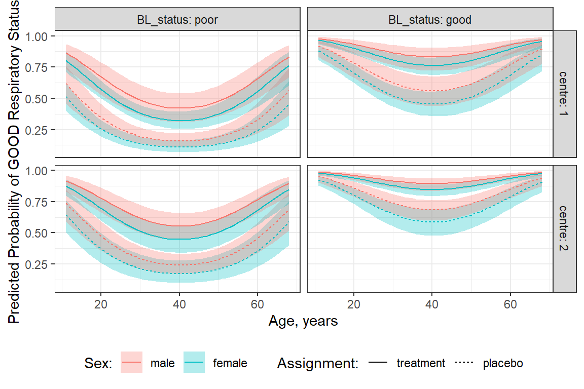
16.5.6.3 Females in Center 1
This example uses default settings.
interactions::interact_plot(model = resp_geeglm_ex,
                            pred = age,
                            modx = treatment,
                            mod2 = BL_status,
                            at = list(sex = "female",
centre = "1")) 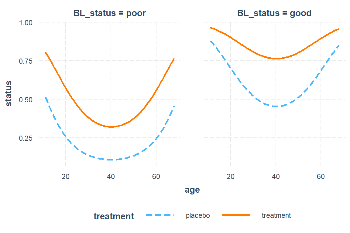
16.5.6.4 Males in Center 2
This example is more preped for publication.
interactions::interact_plot(model = resp_geeglm_ex,
                            pred = age,
                            modx = treatment,
                            mod2 = BL_status,
                            at = list(sex = "male",
                                      centre = "2"),
                            x.label = "Age in Years",
                            y.label = "Predicted Probability of 'Good' Respiratory Status",
                            legend.main = "Intervention: ",
                            mod2.labels = c("Poor at Baseline",
                                            "Good at Baseline"),
                            colors = rep("black", times = 2)) +
  theme_bw() +
  theme(legend.position = c(1, 0),
        legend.justification = c(1.1, -0.1),
        legend.background = element_rect(color = "black"),
        legend.key.width = unit(1.5, "cm")) +
  labs(caption = "Note: Probibilities shown are specific to males at center 2")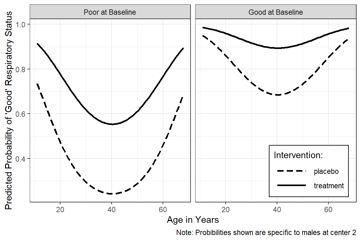
resp_geeglm_ex %>%
  emmeans::emmeans(~ centre + treatment + sex + age + BL_status,
                   at = list(age = seq(from = 11, to = 68, by = 1),
                             sex = "male",
                             centre = "2"),
                   type = "response",
                   level = .68) %>%
  data.frame() %>%
  ggplot(aes(x = age,
             y = prob,
             group = interaction(sex, treatment))) +
  geom_ribbon(aes(ymin = asymp.LCL,
                  ymax = asymp.UCL),
              alpha = .2) +
  geom_line(aes(linetype = fct_rev(treatment))) +
  theme_bw() +
  facet_grid(~ BL_status) +
  labs(x = "Age, years",
       y = "Predicted Probability of\nGOOD Respiratory Status",
       color = "Sex:",
       fill = "Sex:",
       linetype = "Assignment:") +
  theme(legend.position = "bottom")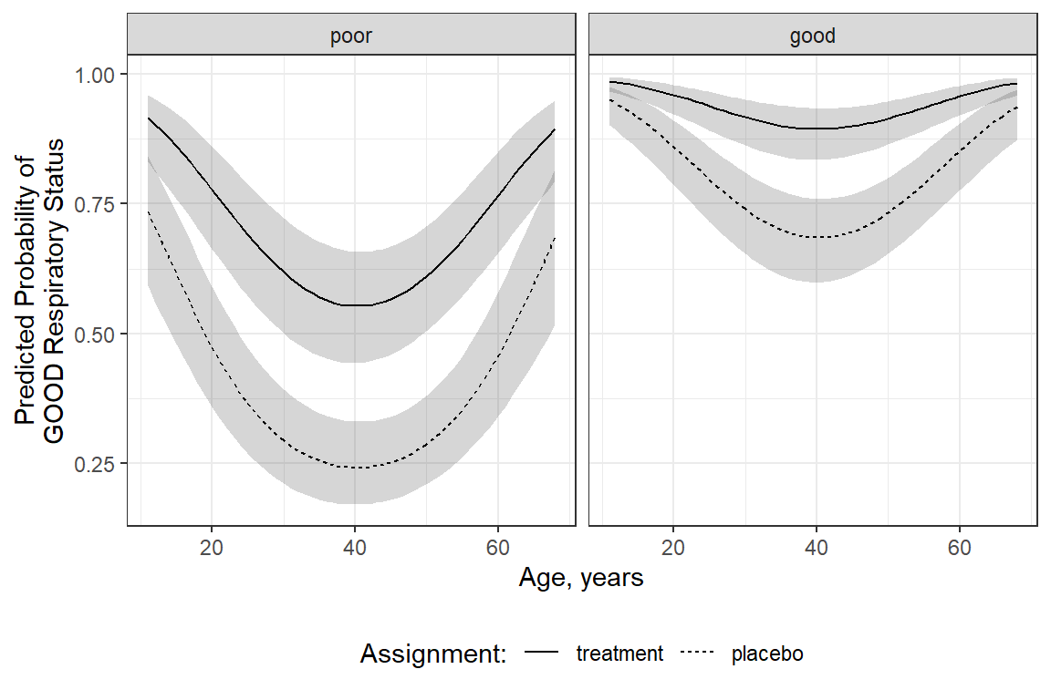
16.6 Conclusion
The Research Question
The question of interest is to assess whether the treatment is effective and to estimate its effect.
The Conclusion
After accounting for baseline status, age, sex and center, participants in the active treatment group had nearly four times higher odds of having ‘good’ respiratory status, when compared to the placebo, exp(b) = 3.881, p<.001, 95% CI [1.85, 8.14].