21 GLMM, Count Outcome: Bolous
GLMM FAQ by: Ben Bolker and others
21.1 Packages
21.1.1 CRAN
library(tidyverse)    # all things tidy
library(pander)       # nice looking genderal tabulations
library(furniture)    # nice table1() descriptives
library(texreg)       # Convert Regression Output to LaTeX or HTML Tables
library(psych)        # contains some useful functions, like headTail

library(lme4)         # Linear, generalized linear, & nonlinear mixed models
library(gee)          # Generalized Estimating Equations
library(optimx)       # Optimizers for use in lme4::glmer
library(MuMIn)        # Multi-Model Inference (caluclate QIC)
library(effects)      # Plotting estimated marginal means
library(interactions)
library(performance)

library(patchwork) # combining graphics21.2 Data Prep
Bolus data from Weiss 2005
Patient controlled analgesia (PCA) comparing 2 dosing regimes to self-control pain
The dataset has the number of requests per interval in 12 successive four-hourly intervals following abdominal surgery for 65 patients in a clinical trial to compare two groups (bolus/lock-out combinations).
Bolus= Large dose of medication given (usually intravenously by direct infusion injection or gravity drip) to raise blood-level concentrations to a therapeutic level
A ‘lock-out’ period followed each dose, where subject may not administer more medication.
- Lock-out time is twice as long in 2mg/dose group
- Allows for max of 30 dosages in 2mg/dose and 60 in 1mg/dose group in any 4-hour period
- No responses neared these upper limits
Variable List:
Indicators
idunique subject indicatortime11 consecutive 4-hour periods: 0, 1, 2, …, 10
Outcome or dependent variable
count# doses recorded for in that 4-hour period
Main predictor or independent variable of interest
group1mg/dose group, 2mg/dose group
21.2.1 Import
data_raw <- read.table("https://raw.githubusercontent.com/CEHS-research/data/master/MLM/bolus.txt",
header = TRUE)str(data_raw) # see the structure'data.frame': 715 obs. of 4 variables:
$ id : int 1 1 1 1 1 1 1 1 1 1 ...
$ group: chr "1mg" "1mg" "1mg" "1mg" ...
$ time : int 0 1 2 3 4 5 6 7 8 9 ...
$ count: int 2 2 5 2 4 0 2 4 4 4 ...psych::headTail(data_raw) id group time count
1 1 1mg 0 2
2 1 1mg 1 2
3 1 1mg 2 5
4 1 1mg 3 2
... ... <NA> ... ...
712 65 2mg 7 6
713 65 2mg 8 1
714 65 2mg 9 2
715 65 2mg 10 021.2.2 Long Format
data_long <- data_raw %>%
  dplyr::mutate(id = factor(id)) %>%
  dplyr::mutate(timeF = factor(time)) %>%
dplyr::mutate(group = factor(group))str(data_long) # see the structure'data.frame': 715 obs. of 5 variables:
$ id : Factor w/ 65 levels "1","2","3","4",..: 1 1 1 1 1 1 1 1 1 1 ...
$ group: Factor w/ 2 levels "1mg","2mg": 1 1 1 1 1 1 1 1 1 1 ...
$ time : int 0 1 2 3 4 5 6 7 8 9 ...
$ count: int 2 2 5 2 4 0 2 4 4 4 ...
$ timeF: Factor w/ 11 levels "0","1","2","3",..: 1 2 3 4 5 6 7 8 9 10 ...psych::headTail(data_long) id group time count timeF
1 1 1mg 0 2 0
2 1 1mg 1 2 1
3 1 1mg 2 5 2
4 1 1mg 3 2 3
... <NA> <NA> ... ... <NA>
712 65 2mg 7 6 7
713 65 2mg 8 1 8
714 65 2mg 9 2 9
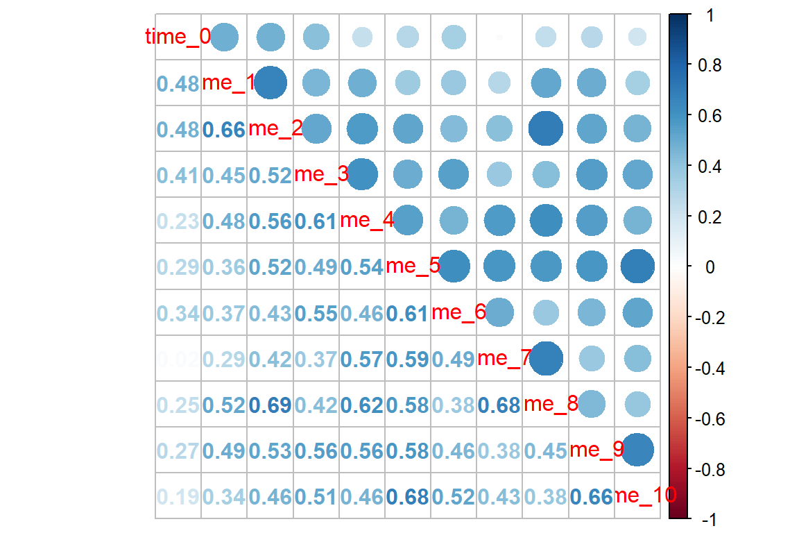
715 65 2mg 10 0 1021.2.3 Wide Format
data_wide <- data_long %>%
  dplyr::select(-timeF) %>%
  tidyr::pivot_wider(names_from = time,
                     names_prefix = "time_",
                     values_from = count)

str(data_wide) # see the structure
tibble [65 × 13] (S3: tbl_df/tbl/data.frame)
$ id : Factor w/ 65 levels "1","2","3","4",..: 1 2 3 4 5 6 7 8 9 10 ...
$ group : Factor w/ 2 levels "1mg","2mg": 1 1 1 1 1 1 1 1 1 1 ...
$ time_0 : int [1:65] 2 3 4 1 7 6 4 2 10 0 ...
$ time_1 : int [1:65] 2 5 8 4 7 5 7 10 9 7 ...
$ time_2 : int [1:65] 5 4 4 3 6 4 4 8 8 1 ...
$ time_3 : int [1:65] 2 4 3 3 8 8 8 17 9 9 ...
$ time_4 : int [1:65] 4 5 12 3 6 7 4 4 4 8 ...
$ time_5 : int [1:65] 0 0 1 1 5 4 4 2 2 0 ...
$ time_6 : int [1:65] 2 6 0 7 4 6 3 6 6 1 ...
$ time_7 : int [1:65] 4 3 6 5 7 5 1 8 1 5 ...
$ time_8 : int [1:65] 4 2 5 0 2 2 3 9 8 4 ...
$ time_9 : int [1:65] 4 7 3 1 5 4 4 1 5 1 ...
$ time_10: int [1:65] 2 4 5 1 0 4 6 4 5 0 ...psych::headTail(data_wide) id group time_0 time_1 time_2 time_3 time_4 time_5 time_6 time_7 time_8
1 1 1mg 2 2 5 2 4 0 2 4 4
2 2 1mg 3 5 4 4 5 0 6 3 2
3 3 1mg 4 8 4 3 12 1 0 6 5
4 4 1mg 1 4 3 3 3 1 7 5 0
5 <NA> <NA> ... ... ... ... ... ... ... ... ...
6 62 2mg 0 13 7 9 19 4 5 11 10
7 63 2mg 11 7 6 9 3 4 6 6 6
8 64 2mg 8 4 22 11 16 4 5 9 12
9 65 2mg 2 2 2 4 4 3 7 6 1
time_9 time_10
1 4 2
2 7 4
3 3 5
4 1 1
5 ... ...
6 6 9
7 6 0
8 12 7
9 2 021.3 Exploratory Data Analysis
21.3.1 Summary Statistics
21.3.1.1 Demographics and Baseline
data_wide %>%
  dplyr::group_by(group) %>%
  furniture::table1("Count at Baseline" = time_0,
                    total   = TRUE,
                    test    = TRUE,
                    na.rm   = FALSE,
                    digits  = 2,
output = "markdown")| Total | 1mg | 2mg | P-Value | |
|---|---|---|---|---|
| n = 65 | n = 30 | n = 35 | ||
| Count at Baseline | 0.448 | |||
| 6.03 (5.17) | 5.50 (4.70) | 6.49 (5.58) |
21.3.1.2 Status over Time
data_wide %>%
  dplyr::group_by(group) %>%
  furniture::table1(time_0,
                    time_1, time_2, time_3, time_4, time_5,
                    time_6, time_7, time_8, time_9, time_10,
                    total   = TRUE,
                    test    = TRUE,
                    na.rm   = FALSE,
                    digits  = 2,
output = "markdown")| Total | 1mg | 2mg | P-Value | |
|---|---|---|---|---|
| n = 65 | n = 30 | n = 35 | ||
| time_0 | 0.448 | |||
| 6.03 (5.17) | 5.50 (4.70) | 6.49 (5.58) | ||
| time_1 | 0.127 | |||
| 6.74 (6.37) | 5.43 (4.00) | 7.86 (7.75) | ||
| time_2 | 0.005 | |||
| 7.37 (6.25) | 5.13 (4.13) | 9.29 (7.12) | ||
| time_3 | 0.165 | |||
| 8.68 (5.94) | 7.57 (5.01) | 9.63 (6.56) | ||
| time_4 | 0.084 | |||
| 6.43 (4.74) | 5.33 (3.36) | 7.37 (5.54) | ||
| time_5 | 0.024 | |||
| 5.37 (4.80) | 3.93 (4.19) | 6.60 (5.00) | ||
| time_6 | 0.052 | |||
| 4.82 (4.16) | 3.73 (3.04) | 5.74 (4.78) | ||
| time_7 | 0.73 | |||
| 4.77 (3.62) | 4.60 (3.16) | 4.91 (4.01) | ||
| time_8 | 0.236 | |||
| 5.69 (4.75) | 4.93 (3.63) | 6.34 (5.51) | ||
| time_9 | 0.008 | |||
| 4.98 (4.43) | 3.50 (2.06) | 6.26 (5.45) | ||
| time_10 | 0.034 | |||
| 4.77 (4.80) | 3.47 (2.83) | 5.89 (5.81) |
21.3.2 Visualize
21.3.2.1 Person Profile Plots, by Group
data_long %>%
  ggplot(aes(x = time,
             y = count)) +
  geom_line(aes(group = id),
            color = "black",
            alpha = .4) +
  facet_grid(. ~ group) +
  theme_bw()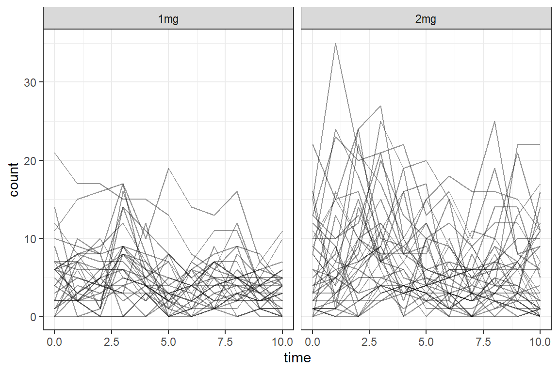
data_long %>%
  ggplot(aes(x = time,
             y = count)) +
  geom_smooth(aes(group = id),
              method = "lm",
              color = "gray",
              se = FALSE) +
  facet_grid(. ~ group) +
  theme_bw()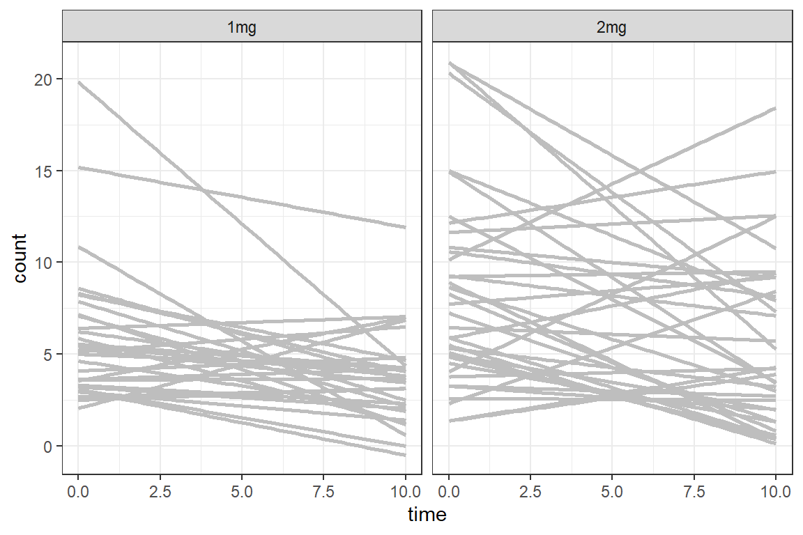
data_long %>%
  ggplot(aes(x = time,
             y = count)) +
  geom_smooth(aes(group = id),
              method = "lm",
              formula = y ~ poly(x, 2),
              color = "gray",
              se = FALSE) +
  facet_grid(. ~ group) +
  theme_bw()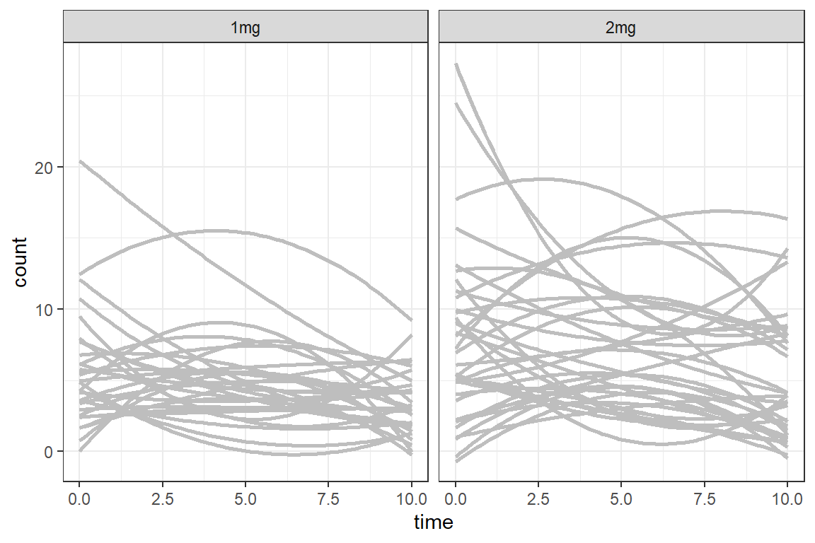
data_long %>%
  ggplot(aes(x = time,
             y = count)) +
  geom_line(aes(group = id)) +
  geom_smooth(method = "loess",
              color = "blue",
              se = FALSE) +
  geom_smooth(method = "lm",
              color = "red",
              se = FALSE) +
  facet_grid(. ~ group) +
  theme_bw()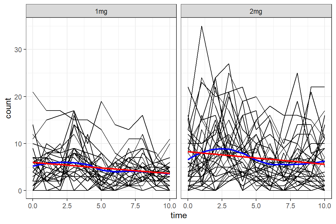
data_long %>%
  ggplot(aes(x = time,
             y = log(count + .1))) +
  geom_line(aes(group = id)) +
  geom_smooth(method = "loess",
              color = "blue",
              se = FALSE) +
  geom_smooth(method = "lm",
              color = "red",
              se = FALSE) +
  facet_grid(. ~ group) +
  theme_bw()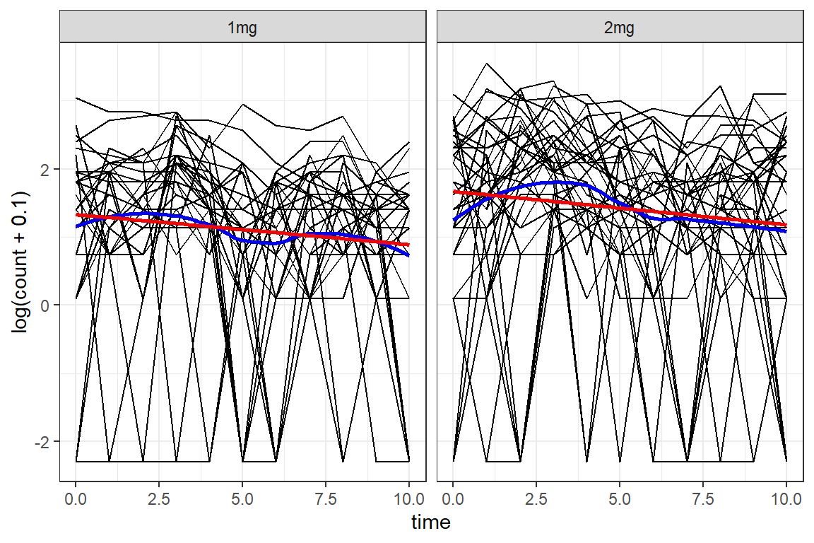
data_long %>%
  ggplot(aes(x = time,
             y = count)) +
  geom_smooth(aes(color = "1. Loess"),
              method = "loess",
              se = FALSE) +
  geom_smooth(aes(color = "2. Linear"),
              method = "lm",
              se = FALSE) +
  geom_smooth(aes(color = "3. Quadratic"),
              method = "lm",
              formula = y ~ poly(x, 2),
              se = FALSE) +
  geom_smooth(aes(color = "4. Cubic"),
              method = "lm",
              formula = y ~ poly(x, 3),
              se = FALSE) +
  facet_grid(. ~ group) +
  theme_bw() +
  labs(color = "Type of Smoother") +
  theme(legend.position = "bottom",
        legend.key.width = unit(1.5, "cm"))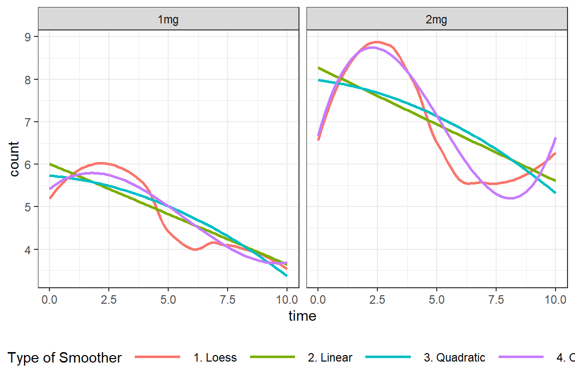
21.3.2.2 Means over Time, BY Group
data_long %>%
  dplyr::group_by(group, timeF) %>%
  dplyr::summarise(M = mean(count)) %>%
  ggplot(aes(x = timeF,
             y = M,
             group = group,
             color = group)) +
  geom_point() +
  geom_line() +
  theme_bw() +
  labs(x = "Four-week Intervals",
       y = "Sample Mean Count",
color = "Dose") 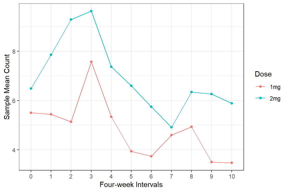
data_long %>%
  dplyr::group_by(group, timeF) %>%
  dplyr::summarise(M = mean(log(count + .1))) %>%
  ggplot(aes(x = timeF,
             y = M,
             group = group,
             color = group)) +
  geom_point() +
  geom_line() +
  theme_bw() +
  labs(x = "Four-week Intervals",
       y = "Sample Mean Count",
color = "Dose") 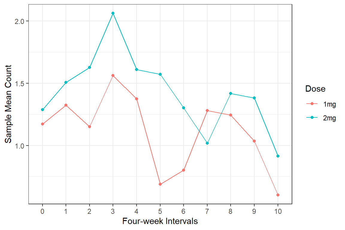
21.4 GEE Analysis
21.4.1 Fit Various Correlation Structures
21.4.1.1 Exchangable
mod_gee_ex <- gee::gee(count ~ group + time + I(time^2),
                       id = id,
                       data = data_long,
                       family = poisson(link = "log"),
                       corstr = 'exchangeable')
(Intercept) group2mg time I(time^2)
1.721889 0.362804 -0.002225 -0.004167 summary(mod_gee_ex)
 GEE:  GENERALIZED LINEAR MODELS FOR DEPENDENT DATA
 gee S-function, version 4.13 modified 98/01/27 (1998)

Model:
 Link:                      Logarithm
 Variance to Mean Relation: Poisson
 Correlation Structure:     Exchangeable

Call:
gee::gee(formula = count ~ group + time + I(time^2), id = id,
    data = data_long, family = poisson(link = "log"), corstr = "exchangeable")

Summary of Residuals:
    Min      1Q  Median      3Q     Max
-7.9757 -3.5612 -0.9249  2.1911 27.0751


Coefficients:
             Estimate Naive S.E.  Naive z Robust S.E. Robust z
(Intercept)  1.733829   0.120291 14.41360    0.117644 14.73794
group2mg     0.342576   0.140827  2.43261    0.140090  2.44539
time        -0.002224   0.026992 -0.08239    0.030992 -0.07175
I(time^2)   -0.004168   0.002689 -1.55019    0.002734 -1.52491

Estimated Scale Parameter:  3.989
Number of Iterations:  2

Working Correlation
        [,1]   [,2]   [,3]   [,4]   [,5]   [,6]   [,7]   [,8]   [,9]  [,10]
 [1,] 1.0000 0.4179 0.4179 0.4179 0.4179 0.4179 0.4179 0.4179 0.4179 0.4179
 [2,] 0.4179 1.0000 0.4179 0.4179 0.4179 0.4179 0.4179 0.4179 0.4179 0.4179
 [3,] 0.4179 0.4179 1.0000 0.4179 0.4179 0.4179 0.4179 0.4179 0.4179 0.4179
 [4,] 0.4179 0.4179 0.4179 1.0000 0.4179 0.4179 0.4179 0.4179 0.4179 0.4179
 [5,] 0.4179 0.4179 0.4179 0.4179 1.0000 0.4179 0.4179 0.4179 0.4179 0.4179
 [6,] 0.4179 0.4179 0.4179 0.4179 0.4179 1.0000 0.4179 0.4179 0.4179 0.4179
 [7,] 0.4179 0.4179 0.4179 0.4179 0.4179 0.4179 1.0000 0.4179 0.4179 0.4179
 [8,] 0.4179 0.4179 0.4179 0.4179 0.4179 0.4179 0.4179 1.0000 0.4179 0.4179
 [9,] 0.4179 0.4179 0.4179 0.4179 0.4179 0.4179 0.4179 0.4179 1.0000 0.4179
[10,] 0.4179 0.4179 0.4179 0.4179 0.4179 0.4179 0.4179 0.4179 0.4179 1.0000
[11,] 0.4179 0.4179 0.4179 0.4179 0.4179 0.4179 0.4179 0.4179 0.4179 0.4179
       [,11]
 [1,] 0.4179
 [2,] 0.4179
 [3,] 0.4179
 [4,] 0.4179
 [5,] 0.4179
 [6,] 0.4179
 [7,] 0.4179
 [8,] 0.4179
 [9,] 0.4179
[10,] 0.4179
[11,] 1.0000
21.4.1.2 Auto-regressive (correlation decay over time)
mod_gee_ar <- gee::gee(count ~ group + time + I(time^2),
                       id = id,
                       data = data_long,
                       family = poisson(link = "log"),
                       corstr = "AR-M",
                       Mv = 1)
(Intercept) group2mg time I(time^2)
1.721889 0.362804 -0.002225 -0.004167 summary(mod_gee_ar)
 GEE:  GENERALIZED LINEAR MODELS FOR DEPENDENT DATA
 gee S-function, version 4.13 modified 98/01/27 (1998)

Model:
 Link:                      Logarithm
 Variance to Mean Relation: Poisson
 Correlation Structure:     AR-M , M = 1

Call:
gee::gee(formula = count ~ group + time + I(time^2), id = id,
    data = data_long, family = poisson(link = "log"), corstr = "AR-M",
    Mv = 1)

Summary of Residuals:
    Min      1Q  Median      3Q     Max
-7.6777 -3.5564 -0.9632  2.3223 27.3599


Coefficients:
             Estimate Naive S.E. Naive z Robust S.E. Robust z
(Intercept)  1.661182   0.114381 14.5232    0.122138  13.6009
group2mg     0.355589   0.105265  3.3780    0.136941   2.5967
time         0.022501   0.042041  0.5352    0.032654   0.6891
I(time^2)   -0.005865   0.004118 -1.4242    0.002939  -1.9959

Estimated Scale Parameter:  4.009
Number of Iterations:  2

Working Correlation
          [,1]     [,2]     [,3]    [,4]    [,5]    [,6]    [,7]    [,8]
 [1,] 1.000000 0.533655 0.284788 0.15198 0.08110 0.04328 0.02310 0.01233
 [2,] 0.533655 1.000000 0.533655 0.28479 0.15198 0.08110 0.04328 0.02310
 [3,] 0.284788 0.533655 1.000000 0.53366 0.28479 0.15198 0.08110 0.04328
 [4,] 0.151978 0.284788 0.533655 1.00000 0.53366 0.28479 0.15198 0.08110
 [5,] 0.081104 0.151978 0.284788 0.53366 1.00000 0.53366 0.28479 0.15198
 [6,] 0.043282 0.081104 0.151978 0.28479 0.53366 1.00000 0.53366 0.28479
 [7,] 0.023097 0.043282 0.081104 0.15198 0.28479 0.53366 1.00000 0.53366
 [8,] 0.012326 0.023097 0.043282 0.08110 0.15198 0.28479 0.53366 1.00000
 [9,] 0.006578 0.012326 0.023097 0.04328 0.08110 0.15198 0.28479 0.53366
[10,] 0.003510 0.006578 0.012326 0.02310 0.04328 0.08110 0.15198 0.28479
[11,] 0.001873 0.003510 0.006578 0.01233 0.02310 0.04328 0.08110 0.15198
          [,9]    [,10]    [,11]
 [1,] 0.006578 0.003510 0.001873
 [2,] 0.012326 0.006578 0.003510
 [3,] 0.023097 0.012326 0.006578
 [4,] 0.043282 0.023097 0.012326
 [5,] 0.081104 0.043282 0.023097
 [6,] 0.151978 0.081104 0.043282
 [7,] 0.284788 0.151978 0.081104
 [8,] 0.533655 0.284788 0.151978
 [9,] 1.000000 0.533655 0.284788
[10,] 0.533655 1.000000 0.533655
[11,] 0.284788 0.533655 1.000000
21.4.1.3 Unstructured
mod_gee_un <- gee::gee(count ~ group + time + I(time^2),
                       id = id,
                       data = data_long,
                       family = poisson(link = "log"),
                       corstr = "unstructured")
(Intercept) group2mg time I(time^2)
1.721889 0.362804 -0.002225 -0.004167 summary(mod_gee_un)
 GEE:  GENERALIZED LINEAR MODELS FOR DEPENDENT DATA
 gee S-function, version 4.13 modified 98/01/27 (1998)

Model:
 Link:                      Logarithm
 Variance to Mean Relation: Poisson
 Correlation Structure:     Unstructured

Call:
gee::gee(formula = count ~ group + time + I(time^2), id = id,
    data = data_long, family = poisson(link = "log"), corstr = "unstructured")

Summary of Residuals:
    Min      1Q  Median      3Q     Max
-6.6661 -2.6978 -0.2413  2.9980 28.4379


Coefficients:
             Estimate Naive S.E. Naive z Robust S.E. Robust z
(Intercept)  1.562649   0.136816  11.422    0.135840   11.504
group2mg     0.284092   0.151482   1.875    0.141552    2.007
time         0.043984   0.031621   1.391    0.040017    1.099
I(time^2)   -0.009419   0.002544  -3.703    0.003708   -2.540

Estimated Scale Parameter:  4.884
Number of Iterations:  11

Working Correlation
         [,1]   [,2]   [,3]   [,4]   [,5]   [,6]   [,7]    [,8]   [,9]  [,10]
 [1,] 1.00000 0.5364 0.5054 0.4452 0.1958 0.2503 0.2412 0.01557 0.2516 0.2408
 [2,] 0.53641 1.0000 0.8486 0.6189 0.4691 0.3295 0.3091 0.22892 0.6117 0.5272
 [3,] 0.50543 0.8486 1.0000 0.6950 0.5126 0.4635 0.3188 0.29785 0.7877 0.5554
 [4,] 0.44520 0.6189 0.6950 1.0000 0.6056 0.4314 0.4065 0.31539 0.6111 0.6445
 [5,] 0.19583 0.4691 0.5126 0.6056 1.0000 0.3786 0.2775 0.35148 0.5374 0.4410
 [6,] 0.25027 0.3295 0.4635 0.4314 0.3786 1.0000 0.4126 0.37182 0.4792 0.4416
 [7,] 0.24115 0.3091 0.3188 0.4065 0.2775 0.4126 1.0000 0.28205 0.2613 0.2911
 [8,] 0.01557 0.2289 0.2979 0.3154 0.3515 0.3718 0.2820 1.00000 0.4936 0.2334
 [9,] 0.25156 0.6117 0.7877 0.6111 0.5374 0.4792 0.2613 0.49357 1.0000 0.4560
[10,] 0.24084 0.5272 0.5554 0.6445 0.4410 0.4416 0.2911 0.23340 0.4560 1.0000
[11,] 0.21857 0.4445 0.5932 0.7372 0.4356 0.6329 0.4043 0.32292 0.4933 0.7378
       [,11]
 [1,] 0.2186
 [2,] 0.4445
 [3,] 0.5932
 [4,] 0.7372
 [5,] 0.4356
 [6,] 0.6329
 [7,] 0.4043
 [8,] 0.3229
 [9,] 0.4933
[10,] 0.7378
[11,] 1.0000
21.4.2 Compare Corelation Structures
21.4.2.1 QIC: Model Fit
MuMIn::model.sel(mod_gee_ex,
                 mod_gee_ar,
                 mod_gee_un,
                 rank = "QIC")    #sorts the best to the TOP, uses QIC(I) to choose corelation structure
Model selection table
(Intrc) group time time^2 corstr Mv qLik QIC delta weight
mod_gee_ex 1.734 + -0.002224 -0.004168 ex 3464 -6904 0.00 0.432
mod_gee_ar 1.661 + 0.022500 -0.005865 AR-M 1 3462 -6904 0.18 0.395
mod_gee_un 1.563 + 0.043980 -0.009419 un 3407 -6902 1.83 0.173
Abbreviations:
corstr: ex = 'exchangeable', un = 'unstructured'
Models ranked by QIC(x) performance::compare_performance(mod_gee_ex,
mod_gee_ar,
mod_gee_un,
rank = TRUE)# Comparison of Model Performance Indices
Name | Model | RMSE | Sigma | Score_log | Score_spherical | Performance-Score
------------------------------------------------------------------------------------
mod_gee_ex | gee | 4.996 | 5.010 | -3.535 | 0.030 | 76.57%
mod_gee_ar | gee | 4.998 | 5.012 | -3.537 | 0.030 | 72.74%
mod_gee_un | gee | 5.081 | 5.096 | -3.614 | 0.030 | 25.00%21.4.2.2 Model Parameter Table
texreg::knitreg(list(extract_gee_exp(mod_gee_ex),
                     extract_gee_exp(mod_gee_ar),
                     extract_gee_exp(mod_gee_un)),
                custom.model.names = c("Exchangable",
                                       "AutoRegressive",
                                       "Unstructured"),
                caption = "GEE: Main Effects Only, with Quadratic Time",
                single.row = TRUE,
ci.test = 1)| Exchangable | AutoRegressive | Unstructured | |
|---|---|---|---|
| (Intercept) | 5.66 [4.50; 7.13]* | 5.27 [4.14; 6.69]* | 4.77 [3.66; 6.23]* |
| group2mg | 1.41 [1.07; 1.85]* | 1.43 [1.09; 1.87]* | 1.33 [1.01; 1.75]* |
| time | 1.00 [0.94; 1.06] | 1.02 [0.96; 1.09] | 1.04 [0.97; 1.13] |
| time^2 | 1.00 [0.99; 1.00] | 0.99 [0.99; 1.00]* | 0.99 [0.98; 1.00]* |
| Dispersion | 3.99 | 4.01 | 4.88 |
| * Null hypothesis value outside the confidence interval. | |||
21.4.3 Add Interaction Terms
mod_gee_ar2 <- gee::gee(count ~ group*time + group*I(time^2),
                        id = id,
                        data = data_long,
                        family = poisson(link = "log"),
                        corstr = "AR-M",
                        Mv = 1)
(Intercept) group2mg time I(time^2)
1.7400506 0.3334615 0.0004752 -0.0051756
group2mg:time group2mg:I(time^2)
-0.0040973 0.0015817 summary(mod_gee_ar2)
 GEE:  GENERALIZED LINEAR MODELS FOR DEPENDENT DATA
 gee S-function, version 4.13 modified 98/01/27 (1998)

Model:
 Link:                      Logarithm
 Variance to Mean Relation: Poisson
 Correlation Structure:     AR-M , M = 1

Call:
gee::gee(formula = count ~ group * time + group * I(time^2),
    id = id, data = data_long, family = poisson(link = "log"),
    corstr = "AR-M", Mv = 1)

Summary of Residuals:
    Min      1Q  Median      3Q     Max
-7.5267 -3.4662 -0.7786  2.2661 27.5763


Coefficients:
                     Estimate Naive S.E. Naive z Robust S.E. Robust z
(Intercept)         1.7220483   0.148755 11.5764     0.14094 12.21793
group2mg            0.2568280   0.191465  1.3414     0.19142  1.34172
time                0.0077450   0.068090  0.1137     0.05263  0.14717
I(time^2)          -0.0057086   0.006751 -0.8456     0.00489 -1.16742
group2mg:time       0.0240638   0.086606  0.2779     0.06720  0.35808
group2mg:I(time^2) -0.0002992   0.008524 -0.0351     0.00612 -0.04888

Estimated Scale Parameter:  4.014
Number of Iterations:  3

Working Correlation
          [,1]     [,2]     [,3]    [,4]    [,5]    [,6]    [,7]    [,8]
 [1,] 1.000000 0.534560 0.285754 0.15275 0.08166 0.04365 0.02333 0.01247
 [2,] 0.534560 1.000000 0.534560 0.28575 0.15275 0.08166 0.04365 0.02333
 [3,] 0.285754 0.534560 1.000000 0.53456 0.28575 0.15275 0.08166 0.04365
 [4,] 0.152753 0.285754 0.534560 1.00000 0.53456 0.28575 0.15275 0.08166
 [5,] 0.081655 0.152753 0.285754 0.53456 1.00000 0.53456 0.28575 0.15275
 [6,] 0.043650 0.081655 0.152753 0.28575 0.53456 1.00000 0.53456 0.28575
 [7,] 0.023333 0.043650 0.081655 0.15275 0.28575 0.53456 1.00000 0.53456
 [8,] 0.012473 0.023333 0.043650 0.08166 0.15275 0.28575 0.53456 1.00000
 [9,] 0.006668 0.012473 0.023333 0.04365 0.08166 0.15275 0.28575 0.53456
[10,] 0.003564 0.006668 0.012473 0.02333 0.04365 0.08166 0.15275 0.28575
[11,] 0.001905 0.003564 0.006668 0.01247 0.02333 0.04365 0.08166 0.15275
          [,9]    [,10]    [,11]
 [1,] 0.006668 0.003564 0.001905
 [2,] 0.012473 0.006668 0.003564
 [3,] 0.023333 0.012473 0.006668
 [4,] 0.043650 0.023333 0.012473
 [5,] 0.081655 0.043650 0.023333
 [6,] 0.152753 0.081655 0.043650
 [7,] 0.285754 0.152753 0.081655
 [8,] 0.534560 0.285754 0.152753
 [9,] 1.000000 0.534560 0.285754
[10,] 0.534560 1.000000 0.534560
[11,] 0.285754 0.534560 1.000000MuMIn::QIC(mod_gee_ar,
mod_gee_ar2,
typeR = TRUE) # NOT the default QIC
mod_gee_ar -6900
mod_gee_ar2 -6897texreg::knitreg(list(extract_gee_exp(mod_gee_ar),
extract_gee_exp(mod_gee_ar2)),
single.row = TRUE,
ci.test = 1)<table class="texreg" style="margin: 10px auto;border-collapse: collapse;border-spacing: 0px;caption-side: bottom;color: #000000;border-top: 2px solid #000000;">
<caption>Statistical models</caption>
<thead>
<tr>
<th style="padding-left: 5px;padding-right: 5px;"> </th>
<th style="padding-left: 5px;padding-right: 5px;">Model 1</th>
<th style="padding-left: 5px;padding-right: 5px;">Model 2</th>
</tr>
</thead>
<tbody>
<tr style="border-top: 1px solid #000000;">
<td style="padding-left: 5px;padding-right: 5px;">(Intercept)</td>
<td style="padding-left: 5px;padding-right: 5px;">5.27 [4.14; 6.69]<sup>*</sup></td>
<td style="padding-left: 5px;padding-right: 5px;">5.60 [4.25; 7.38]<sup>*</sup></td>
</tr>
<tr>
<td style="padding-left: 5px;padding-right: 5px;">group2mg</td>
<td style="padding-left: 5px;padding-right: 5px;">1.43 [1.09; 1.87]<sup>*</sup></td>
<td style="padding-left: 5px;padding-right: 5px;">1.29 [0.89; 1.88]</td>
</tr>
<tr>
<td style="padding-left: 5px;padding-right: 5px;">time</td>
<td style="padding-left: 5px;padding-right: 5px;">1.02 [0.96; 1.09]</td>
<td style="padding-left: 5px;padding-right: 5px;">1.01 [0.91; 1.12]</td>
</tr>
<tr>
<td style="padding-left: 5px;padding-right: 5px;">time^2</td>
<td style="padding-left: 5px;padding-right: 5px;">0.99 [0.99; 1.00]<sup>*</sup></td>
<td style="padding-left: 5px;padding-right: 5px;">0.99 [0.98; 1.00]</td>
</tr>
<tr>
<td style="padding-left: 5px;padding-right: 5px;">group2mg:time</td>
<td style="padding-left: 5px;padding-right: 5px;"> </td>
<td style="padding-left: 5px;padding-right: 5px;">1.02 [0.90; 1.17]</td>
</tr>
<tr>
<td style="padding-left: 5px;padding-right: 5px;">group2mg:time^2</td>
<td style="padding-left: 5px;padding-right: 5px;"> </td>
<td style="padding-left: 5px;padding-right: 5px;">1.00 [0.99; 1.01]</td>
</tr>
<tr style="border-top: 1px solid #000000;">
<td style="padding-left: 5px;padding-right: 5px;">Dispersion</td>
<td style="padding-left: 5px;padding-right: 5px;">4.01</td>
<td style="padding-left: 5px;padding-right: 5px;">4.01</td>
</tr>
</tbody>
<tfoot>
<tr>
<td style="font-size: 0.8em;" colspan="3"><sup>*</sup> Null hypothesis value outside the confidence interval.</td>
</tr>
</tfoot>
</table>21.4.4 Visualize Best Model
21.4.4.1 Model Parameter Table
texreg::knitreg(extract_gee_exp(mod_gee_ar),
                caption = "GEE: Final Model (auto regressive)",
                single.row = TRUE,
ci.test = 1)| Model 1 | |
|---|---|
| (Intercept) | 5.27 [4.14; 6.69]* |
| group2mg | 1.43 [1.09; 1.87]* |
| time | 1.02 [0.96; 1.09] |
| time^2 | 0.99 [0.99; 1.00]* |
| Dispersion | 4.01 |
| * 1 outside the confidence interval. | |
21.4.4.2 Refit via geepack::geeglm()
mod_geeglm_ar <- geepack::geeglm(count ~ group + time + I(time^2),
                       id = id,
                       data = data_long,
                       family = poisson(link = "log"),
                       corstr = "ar1")

summary(mod_geeglm_ar)
Call:
geepack::geeglm(formula = count ~ group + time + I(time^2), family = poisson(link = "log"),
    data = data_long, id = id, corstr = "ar1")

 Coefficients:
            Estimate  Std.err   Wald Pr(>|W|)
(Intercept)  1.63046  0.12861 160.71   <2e-16 ***
group2mg     0.34575  0.13880   6.21    0.013 *
time         0.03588  0.03558   1.02    0.313
I(time^2)   -0.00665  0.00321   4.31    0.038 *
---
Signif. codes:  0 '***' 0.001 '**' 0.01 '*' 0.05 '.' 0.1 ' ' 1

Correlation structure = ar1
Estimated Scale Parameters:

            Estimate Std.err
(Intercept)        4   0.435
  Link = identity

Estimated Correlation Parameters:
      Estimate Std.err
alpha    0.775  0.0333
Number of clusters: 65 Maximum cluster size: 11 interactions::interact_plot(model = mod_geeglm_ar,
pred = time,
modx = group)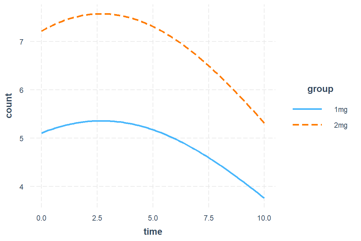
21.4.4.3 Predict over a Grid
Estimated Marginal Mean Counts
expand.grid(time = 0:10,
            group = levels(data_long$group)) %>%
  dplyr::mutate(fit = predict(mod_geeglm_ar,
                              newdata = .,
                              type = "response")) %>%
  tidyr::spread(key = group,
                value = fit)
time 1mg 2mg
1 0 5.11 7.22
2 1 5.26 7.43
3 2 5.34 7.55
4 3 5.36 7.57
5 4 5.30 7.49
6 5 5.17 7.31
7 6 4.98 7.04
8 7 4.74 6.69
9 8 4.44 6.28
10 9 4.11 5.81
11 10 3.76 5.3121.4.4.4 Plot Estimated Marginal Means
expand.grid(time = 0:10,
            group = levels(data_long$group)) %>%
  dplyr::mutate(fit = predict(mod_geeglm_ar,
                              newdata = .,
                              type = "response")) %>%
  ggplot(aes(x = time,
             y = fit,
             color = fct_rev(group))) +
  geom_point() +
  geom_line() +
  theme_bw() +
  labs(x = "Four-week Intervals",
       y = "Estimated Populaton Mean Count",
       color = "Dose") +
  scale_x_continuous(breaks = 0:10)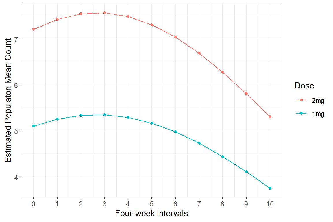
21.5 GLMM Analysis
21.5.1 RI: Random Intercepts Only
mod_glmer_ri <- lme4::glmer(count ~ group + I(time/4) + I((time/4)^2) + (1|id),
                            data = data_long,
                            family = poisson(link = "log"))

summary(mod_glmer_ri)
Generalized linear mixed model fit by maximum likelihood (Laplace
Approximation) [glmerMod]
Family: poisson ( log )
Formula: count ~ group + I(time/4) + I((time/4)^2) + (1 | id)
Data: data_long
AIC BIC logLik deviance df.resid
4061 4083 -2025 4051 710
Scaled residuals:
Min 1Q Median 3Q Max
-3.109 -1.092 -0.150 0.814 5.628
Random effects:
Groups Name Variance Std.Dev.
id (Intercept) 0.283 0.532
Number of obs: 715, groups: id, 65
Fixed effects:
Estimate Std. Error z value Pr(>|z|)
(Intercept) 1.6099 0.1062 15.15 <2e-16 ***
group2mg 0.3110 0.1371 2.27 0.023 *
I(time/4) -0.0089 0.0706 -0.13 0.900
I((time/4)^2) -0.0667 0.0281 -2.37 0.018 *
---
Signif. codes: 0 '***' 0.001 '**' 0.01 '*' 0.05 '.' 0.1 ' ' 1
Correlation of Fixed Effects:
(Intr) grp2mg I(t/4)
group2mg -0.700
I(time/4) -0.276 0.000
I((tm/4)^2) 0.226 0.000 -0.96021.5.2 RIAS: Random Intercepts and Slopes
mod_glmer_rias <- lme4::glmer(count ~ group + I(time/4) + I((time/4)^2) + (I(time/4)|id),
                              data = data_long,
                              family = poisson(link = "log"))

summary(mod_glmer_rias)
Generalized linear mixed model fit by maximum likelihood (Laplace
Approximation) [glmerMod]
Family: poisson ( log )
Formula: count ~ group + I(time/4) + I((time/4)^2) + (I(time/4) | id)
Data: data_long
AIC BIC logLik deviance df.resid
3964 3996 -1975 3950 708
Scaled residuals:
Min 1Q Median 3Q Max
-3.045 -0.927 -0.142 0.682 4.886
Random effects:
Groups Name Variance Std.Dev. Corr
id (Intercept) 0.3147 0.561
I(time/4) 0.0825 0.287 -0.36
Number of obs: 715, groups: id, 65
Fixed effects:
Estimate Std. Error z value Pr(>|z|)
(Intercept) 1.5993 0.1093 14.63 <2e-16 ***
group2mg 0.3002 0.1360 2.21 0.0274 *
I(time/4) 0.0452 0.0807 0.56 0.5751
I((time/4)^2) -0.1035 0.0286 -3.62 0.0003 ***
---
Signif. codes: 0 '***' 0.001 '**' 0.01 '*' 0.05 '.' 0.1 ' ' 1
Correlation of Fixed Effects:
(Intr) grp2mg I(t/4)
group2mg -0.679
I(time/4) -0.363 0.005
I((tm/4)^2) 0.224 0.001 -0.848anova(mod_glmer_ri, mod_glmer_rias)Data: data_long
Models:
mod_glmer_ri: count ~ group + I(time/4) + I((time/4)^2) + (1 | id)
mod_glmer_rias: count ~ group + I(time/4) + I((time/4)^2) + (I(time/4) | id)
npar AIC BIC logLik deviance Chisq Df Pr(>Chisq)
mod_glmer_ri 5 4061 4083 -2025 4051
mod_glmer_rias 7 3964 3996 -1975 3950 100 2 <2e-16 ***
---
Signif. codes: 0 '***' 0.001 '**' 0.01 '*' 0.05 '.' 0.1 ' ' 1texreg::knitreg(list(extract_glmer_exp(mod_glmer_ri),
extract_glmer_exp(mod_glmer_rias)),
custom.model.names = c("Intecepts", "Intercepts and Slopes"),
caption = "GLMM: Compare Random Effects",
single.row = TRUE,
ci.test = 1)| Intecepts | Intercepts and Slopes | |
|---|---|---|
| (Intercept) | 5.00 [4.05; 6.17]* | 4.95 [3.99; 6.15]* |
| group2mg | 1.36 [1.04; 1.79]* | 1.35 [1.03; 1.77]* |
| time/4 | 0.99 [0.86; 1.14] | 1.05 [0.89; 1.23] |
| (time/4)^2 | 0.94 [0.88; 0.99]* | 0.90 [0.85; 0.95]* |
| * Null hypothesis value outside the confidence interval. | ||
21.5.3 RAIS: Add Interaction
See the GLMM - Optimizers page for more information on convergence problems.
mod_glmer_rias2 <- lme4::glmer(count ~ group*I(time/4) + group*I((time/4)^2) + ( I(time/4)|id ),
                              data = data_long,
                              control = glmerControl(optimizer ="Nelder_Mead"),  # convergence issues resolved
family = poisson(link = "log")) anova(mod_glmer_rias, mod_glmer_rias2)Data: data_long
Models:
mod_glmer_rias: count ~ group + I(time/4) + I((time/4)^2) + (I(time/4) | id)
mod_glmer_rias2: count ~ group * I(time/4) + group * I((time/4)^2) + (I(time/4) | id)
npar AIC BIC logLik deviance Chisq Df Pr(>Chisq)
mod_glmer_rias 7 3964 3996 -1975 3950
mod_glmer_rias2 9 3968 4009 -1975 3950 0.14 2 0.9321.5.4 Visualize Best Model
21.5.4.1 Model Parameter Table
texreg::knitreg(list(extract_glmer_exp(mod_glmer_rias)),
                caption = "GLMM: Final Model",
                single.row = TRUE,
ci.test = 1)| Model 1 | |
|---|---|
| (Intercept) | 4.95 [3.99; 6.15]* |
| group2mg | 1.35 [1.03; 1.77]* |
| time/4 | 1.05 [0.89; 1.23] |
| (time/4)^2 | 0.90 [0.85; 0.95]* |
| * 1 outside the confidence interval. | |
interactions::interact_plot(model = mod_glmer_rias,
                            pred = time,
                            modx = group)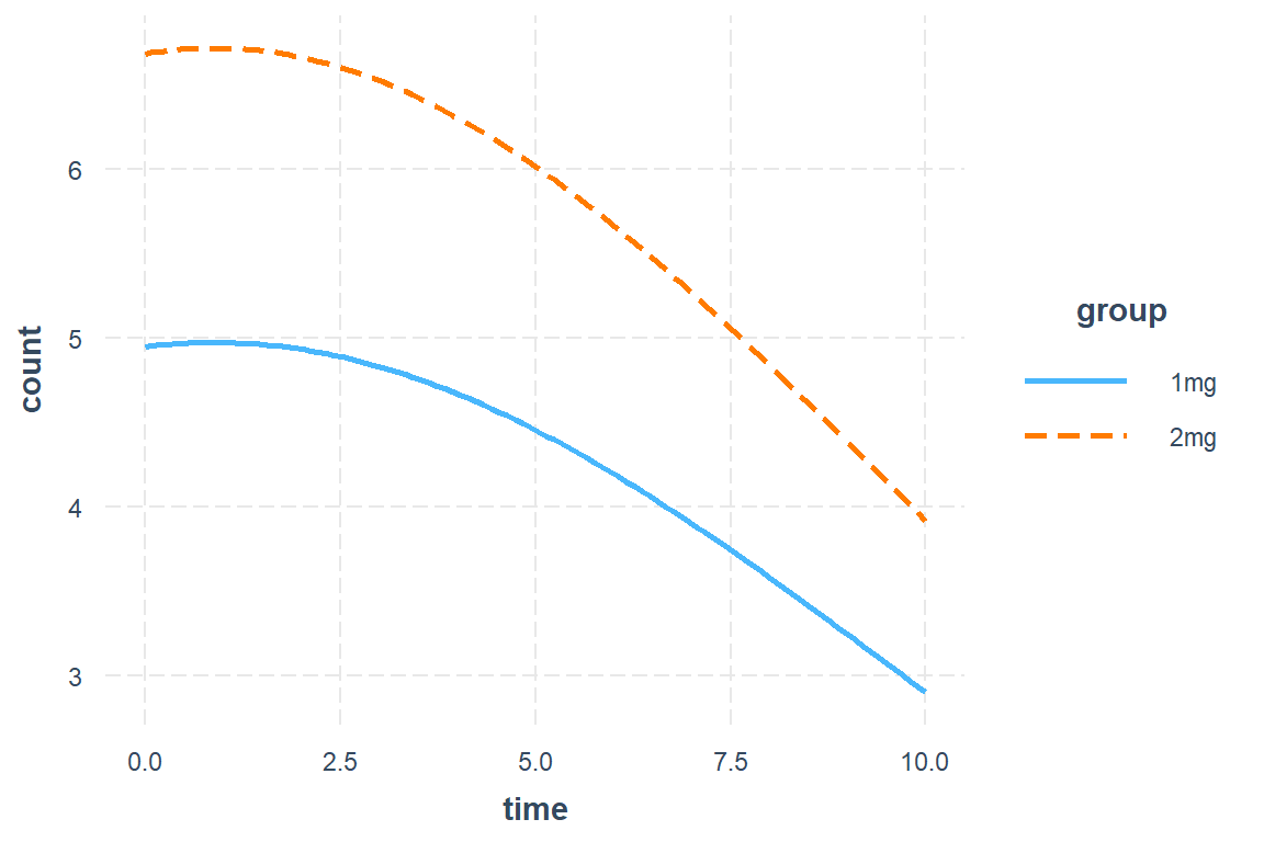
21.5.4.2 Estimated Marginal Means
effects::Effect(focal.predictors = c("group", "time"),
                xlevels = list(time = 0:10),
                mod = mod_glmer_rias) %>%
  data.frame %>%
  dplyr::select(group, time, fit) %>%
  tidyr::spread(key = group,
                value = fit,
                sep = "_")
time group_1mg group_2mg
1 0 4.95 6.68
2 1 4.97 6.71
3 2 4.93 6.66
4 3 4.83 6.52
5 4 4.67 6.30
6 5 4.46 6.02
7 6 4.20 5.67
8 7 3.90 5.27
9 8 3.58 4.84
10 9 3.25 4.38
11 10 2.90 3.9221.5.4.3 Plot Estimated Marginal Means
effects::Effect(focal.predictors = c("group", "time"),
                xlevels = list(time = seq(from = 0, to = 10, by = .25)),
                mod = mod_glmer_rias) %>%
  data.frame %>%
  ggplot(aes(x = time,
             y = fit)) +
  geom_ribbon(aes(ymin = fit - se,
                  ymax = fit + se,
                  fill = group),
              alpha = .3) +
  geom_line(aes(color = group)) +
  theme_bw() +
  labs(x = "Four-week Intervals",
       y = "Estimated Populaton Mean Count",
       color = "Dose",
       fill = "Dose") +
  scale_x_continuous(breaks = 0:10)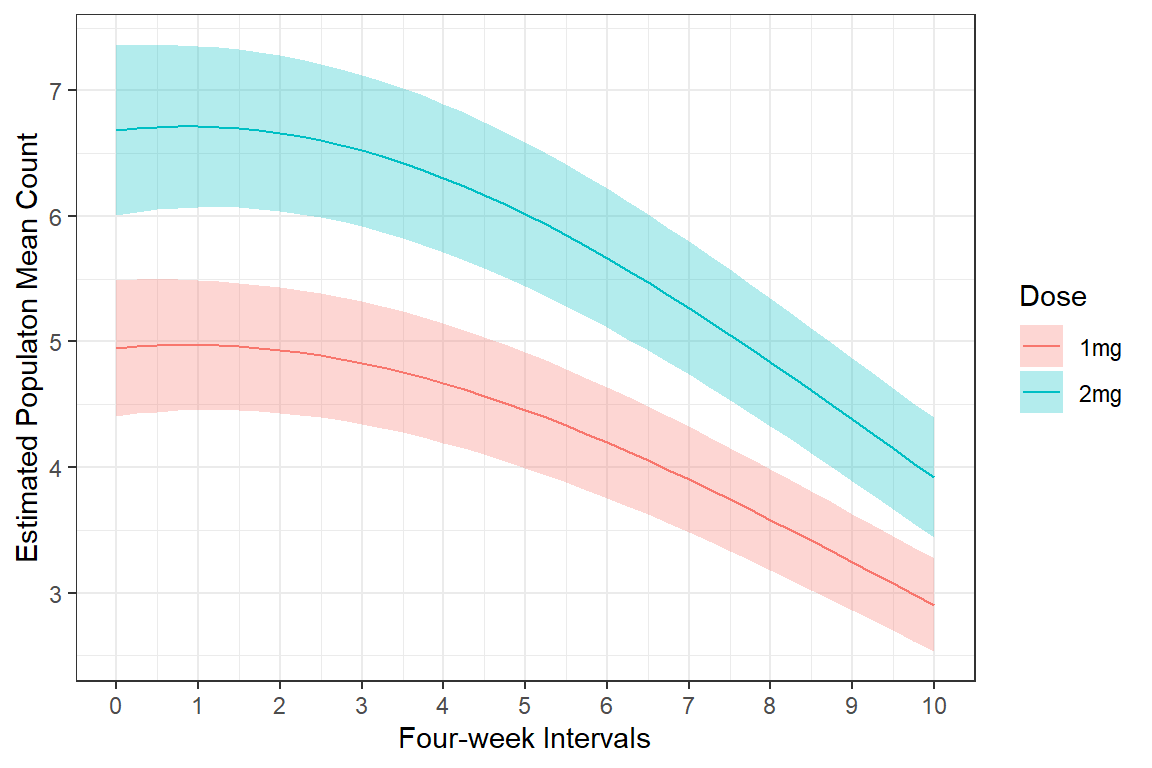
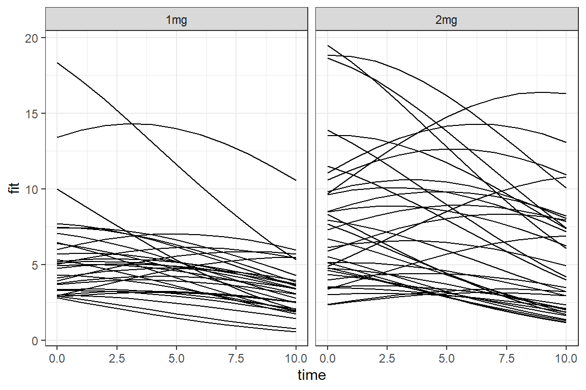
data_long %>%
  dplyr::mutate(fit = predict(mod_glmer_rias,
                              newdata = .,
                              type = "response")) %>%
  ggplot(aes(x = time,
             y = fit)) +
  geom_line(aes(group = id)) +
  facet_grid(.~ group) +
  theme_bw()