18 GEE, Count Outcome: Antibiotics for Leprosy

18.1 Packages

18.1.1 CRAN

library(tidyverse)    # all things tidy
library(pander)       # nice looking genderal tabulations
library(furniture)    # nice table1() descriptives
library(texreg)       # Convert Regression Output to LaTeX or HTML Tables
library(psych)        # contains some useful functions, like headTail

library(interactions)
library(performance)
library(lme4)         # Linear, generalized linear, & nonlinear mixed models

library(corrplot)     # Vizualize correlation matrix
library(gee)          # Genderalized Estimation Equation Solver
library(geepack)      # Genderalized Estimation Equation Package 
library(MuMIn)        # Multi-Model Inference (caluclate QIC)

18.1.2 GitHub

Helper extract functions for exponentiating parameters form generalized regression models within a texreg table of model parameters.

# remotes::install_github("sarbearschwartz/texreghelpr") # first time

library(texreghelpr)

18.2 Background

The following example is presented in the textbook: “Applied Longitudinal Analysis” by Garrett Fitzmaurice, Nan Laird & James Ware

The dataset maybe downloaded from: https://content.sph.harvard.edu/fitzmaur/ala/

Data on count of leprosy bacilli pre- and post-treatment from a clinical trial of antibiotics for leprosy.

Source: Table 14.2.1 (page 422) in Snedecor, G.W. and Cochran, W.G. (1967). Statistical Methods, (6th edn). Ames, Iowa: Iowa State University Press

With permission of Iowa State University Press.

Reference: Snedecor, G.W. and Cochran, W.G. (1967). Statistical Methods, (6th edn). Ames, Iowa: Iowa State University Press

The Background

The dataset consists of count data from a placebo-controlled clinical trial of 30 patients with leprosy at the Eversley Childs Sanitorium in the Philippines. Participants in the study were randomized to either of two antibiotics (denoted treatment drug A and B) or to a placebo (denoted treatment drug C).

Prior to receiving treatment, baseline data on the number of leprosy bacilli at six sites of the body where the bacilli tend to congregate were recorded for each patient. After several months of treatment, the number of leprosy bacilli at six sites of the body were recorded a second time. The outcome variable is the total count of the number of leprosy bacilli at the six sites.

The Research Question

In this study, the question of main scientific interest is whether treatment with antibiotics (drugs A and B) reduces the abundance of leprosy bacilli at the six sites of the body when compared to placebo (drug C).

The Data

Outcome or dependent variable(s)
- count.pre Pre-Treatment Bacilli Count
- count.post Post-Treatment Bacilli Count
Main predictor or independent variable of interest
- drug the treatment group: antibiotics (drugs A and B) or placebo (drug C)

18.2.1 Enter the data by hand!

data_raw <- tibble::tribble(
  ~drug, ~count_pre, ~count_post,
  "A",      11,     6,    "B",       6,     0,    "C",      16,    13,
  "A",       8,     0,    "B",       6,     2,    "C",      13,    10,
  "A",       5,     2,    "B",       7,     3,    "C",      11,    18,
  "A",      14,     8,    "B",       8,     1,    "C",       9,     5,
  "A",      19,    11,    "B",      18,    18,    "C",      21,    23,
  "A",       6,     4,    "B",       8,     4,    "C",      16,    12,
  "A",      10,    13,    "B",      19,    14,    "C",      12,     5,
  "A",       6,     1,    "B",       8,     9,    "C",      12,    16,
  "A",      11,     8,    "B",       5,     1,    "C",       7,     1,
  "A",       3,     0,    "B",      15,     9,    "C",      12,    20)

18.2.2 Wide Format

data_wide <- data_raw %>% 
  dplyr::mutate(drug = factor(drug)) %>% 
  dplyr::mutate(id = row_number()) %>% 
  dplyr::select(id, drug, count_pre, count_post)

str(data_wide)

tibble [30 × 4] (S3: tbl_df/tbl/data.frame)
 $ id        : int [1:30] 1 2 3 4 5 6 7 8 9 10 ...
 $ drug      : Factor w/ 3 levels "A","B","C": 1 2 3 1 2 3 1 2 3 1 ...
 $ count_pre : num [1:30] 11 6 16 8 6 13 5 7 11 14 ...
 $ count_post: num [1:30] 6 0 13 0 2 10 2 3 18 8 ...

psych::headTail(data_wide)

   id drug count_pre count_post
1   1    A        11          6
2   2    B         6          0
3   3    C        16         13
4   4    A         8          0
5 ... <NA>       ...        ...
6  27    C         7          1
7  28    A         3          0
8  29    B        15          9
9  30    C        12         20

18.2.3 Long Format

data_long <- data_wide %>% 
  tidyr::gather(key = obs,
                value = count,
                starts_with("count")) %>% 
  dplyr::mutate(time = case_when(obs == "count_pre" ~ 0,
                                 obs == "count_post" ~ 1)) %>% 
  dplyr::select(id, drug, time, count) %>% 
  dplyr::arrange(id, time)

str(data_long)

tibble [60 × 4] (S3: tbl_df/tbl/data.frame)
 $ id   : int [1:60] 1 1 2 2 3 3 4 4 5 5 ...
 $ drug : Factor w/ 3 levels "A","B","C": 1 1 2 2 3 3 1 1 2 2 ...
 $ time : num [1:60] 0 1 0 1 0 1 0 1 0 1 ...
 $ count: num [1:60] 11 6 6 0 16 13 8 0 6 2 ...

psych::headTail(data_long)

   id drug time count
1   1    A    0    11
2   1    A    1     6
3   2    B    0     6
4   2    B    1     0
5 ... <NA>  ...   ...
6  29    B    0    15
7  29    B    1     9
8  30    C    0    12
9  30    C    1    20

18.3 Exploratory Data Analysis

18.3.1 Summary Statistics

data_long %>% 
  dplyr::group_by(drug, time) %>% 
  dplyr::summarise(N = n(),
                   M = mean(count),
                   VAR = var(count),
                   SD = sd(count)) %>% 
  pander::pander()

summarise() has grouped output by ‘drug’. You can override using the .groups argument.

drug	time	N	M	VAR	SD
A	0	10	9.3	23	4.8
A	1	10	5.3	22	4.6
B	0	10	10.0	28	5.2
B	1	10	6.1	38	6.2
C	0	10	12.9	16	4.0
C	1	10	12.3	51	7.2

18.3.2 Visualize

data_long %>% 
  dplyr::mutate(time_name = case_when(time == 0 ~ "Pre",
                                      time == 1 ~ "Post") %>% 
                  factor(levels = c("Pre", "Post"))) %>% 
  dplyr::mutate(drug_name = fct_recode(drug,
                                       "Antibiotic A" = "A",
                                       "Antibiotic B" = "B",
                                       "Placebo" = "C")) %>% 
  ggplot(aes(x = time_name,
             y = count)) +
  geom_line(aes(group = id)) +
  facet_grid(.~ drug_name) +
  theme_bw() +
  labs(x = NULL,
       y = "Number of Leprosy Bacilli at Six Sites of the Body")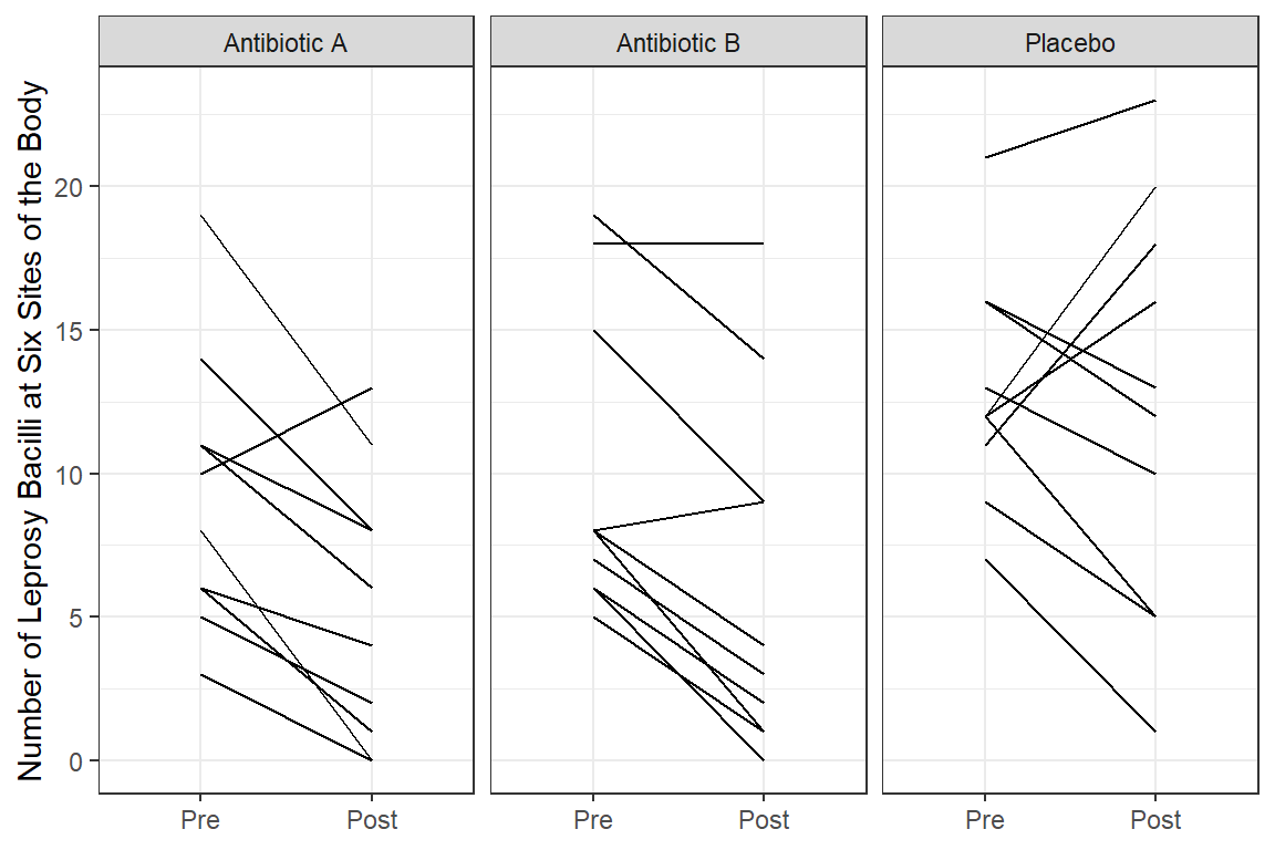

data_long %>% 
  dplyr::mutate(time_name = case_when(time == 0 ~ "Pre",
                                      time == 1 ~ "Post") %>% 
                  factor(levels = c("Pre", "Post"))) %>% 
  dplyr::mutate(drug_name = fct_recode(drug,
                                       "Antibiotic A" = "A",
                                       "Antibiotic B" = "B",
                                       "Placebo" = "C")) %>% 
  ggplot(aes(x = time,
             y = count)) +
  geom_line(aes(group = id),
            color = "gray") +
  geom_smooth(aes(group = drug),
              method = "lm") +
  facet_grid(.~ drug_name) +
  theme_bw() +
  labs(x = NULL,
       y = "Number of Leprosy Bacilli at Six Sites of the Body")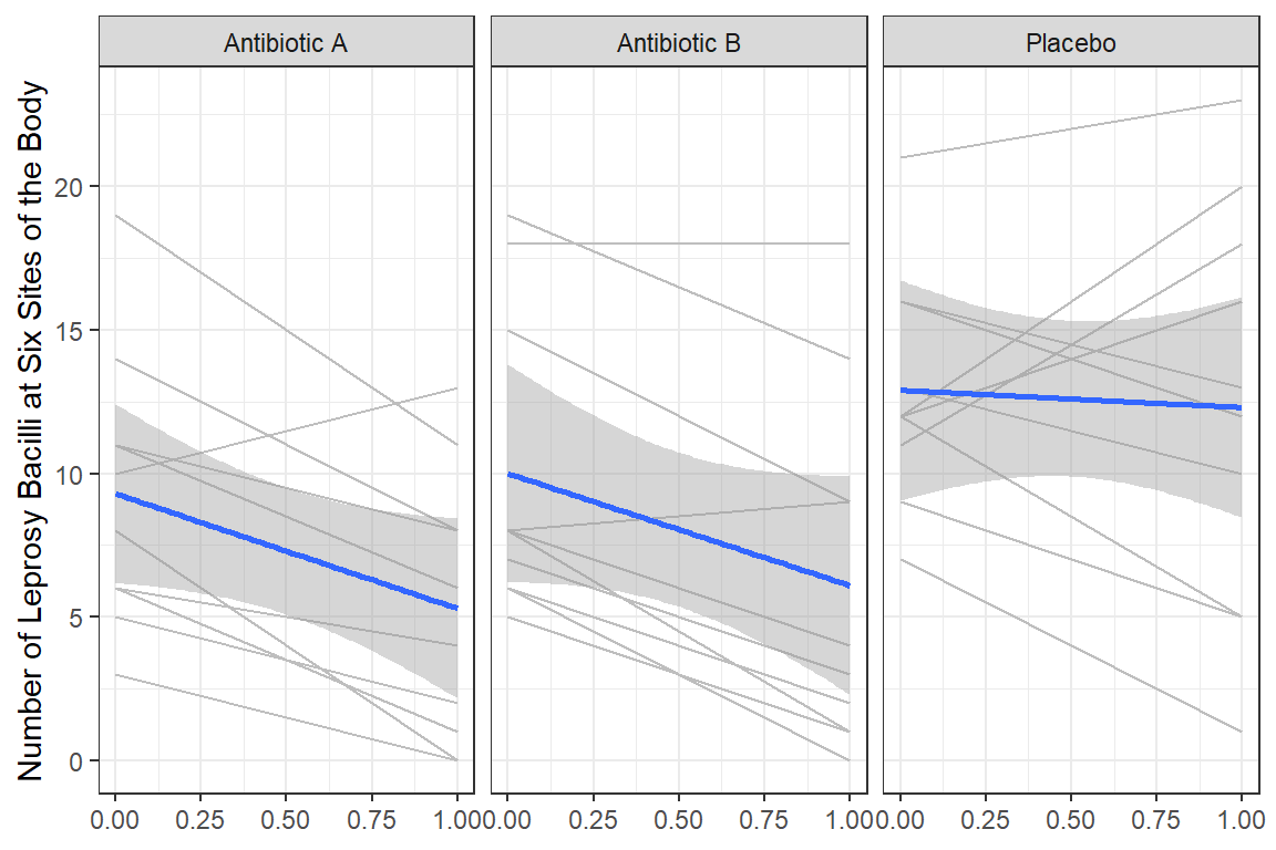

data_long %>% 
  dplyr::mutate(time_name = case_when(time == 0 ~ "Pre",
                                      time == 1 ~ "Post") %>% 
                  factor(levels = c("Pre", "Post"))) %>% 
  dplyr::mutate(drug_name = fct_recode(drug,
                                       "Antibiotic A" = "A",
                                       "Antibiotic B" = "B",
                                       "Placebo" = "C")) %>% 
  ggplot(aes(x = time,
             y = count)) +
  geom_smooth(aes(group = drug,
                  color = drug_name,
                  fill = drug_name),
              method = "lm",
              alpha = .2) +
  theme_bw() +
  labs(x = NULL,
       y = "Number of Leprosy Bacilli at Six Sites of the Body",
       color = NULL,
       fill = NULL) +
  scale_x_continuous(breaks = 0:1,
                     labels = c("Pre-Treatment", "Post-Treatment"))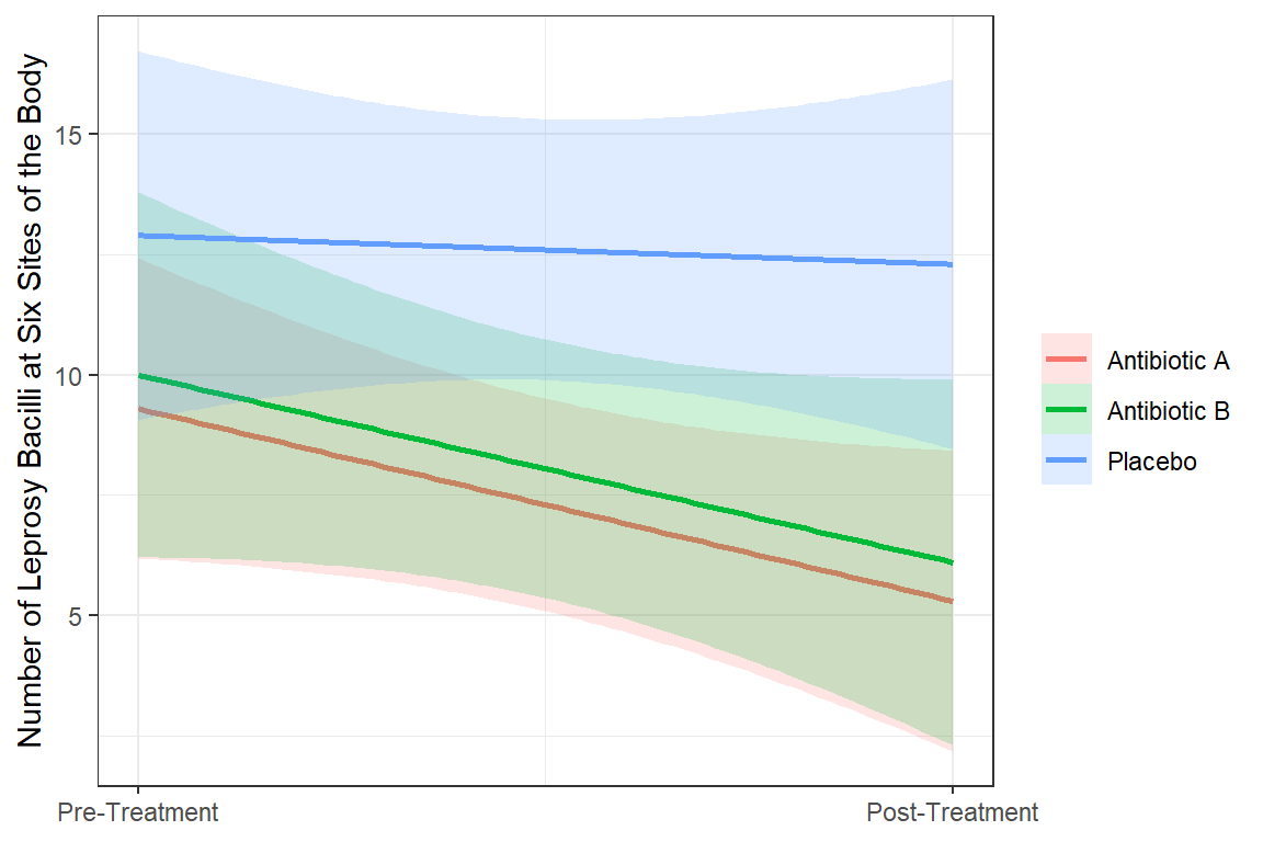

18.4 Generalized Estimating Equations (GEE)

18.4.1 Explore Various Correlation Structures

18.4.1.1 Fit the models - to determine correlation structure

The gee() function in the gee package

mod_gee_ind <- gee::gee(count ~ drug*time,
                        data = data_long,
                        family = poisson(link = "log"),
                        id = id,
                        corstr = "independence")

(Intercept)       drugB       drugC        time  drugB:time  drugC:time 
 2.23001440  0.07257069  0.32721291 -0.56230758  0.06801126  0.51467953

mod_gee_exc <- gee::gee(count ~ drug*time,
                        data = data_long,
                        family = poisson(link = "log"),
                        id = id,
                        corstr = "exchangeable")

(Intercept)       drugB       drugC        time  drugB:time  drugC:time 
 2.23001440  0.07257069  0.32721291 -0.56230758  0.06801126  0.51467953

mod_gee_uns <- gee::gee(count ~ drug*time,
                        data = data_long,
                        family = poisson(link = "log"),
                        id = id,
                        corstr = "unstructured")

(Intercept)       drugB       drugC        time  drugB:time  drugC:time 
 2.23001440  0.07257069  0.32721291 -0.56230758  0.06801126  0.51467953

The GEE models display the robust (sandwich) standard errors.

18.4.1.2 Raw Estimates (Logit Scale)

texreg::knitreg(list(mod_gee_ind, 
                     mod_gee_exc, 
                     mod_gee_uns), 
                custom.model.names = c("Independence",
                                       "Exchangeable",
                                       "Unstructured"),
                single.row = TRUE,
                digits = 3,
                caption = "GEE - Estimates on Log Scale")

GEE - Estimates on Log Scale
	Independence	Exchangeable	Unstructured
(Intercept)	2.230 (0.154)^***	2.230 (0.154)^***	2.230 (0.154)^***
drugB	0.073 (0.220)	0.073 (0.220)	0.073 (0.220)
drugC	0.327 (0.179)	0.327 (0.179)	0.327 (0.179)
time	-0.562 (0.176)^**	-0.562 (0.176)^**	-0.562 (0.176)^**
drugB:time	0.068 (0.246)	0.068 (0.246)	0.068 (0.246)
drugC:time	0.515 (0.221)^*	0.515 (0.221)^*	0.515 (0.221)^*
Scale	3.474	3.474	3.474
Num. obs.	60	60	60
^*p < 0.001; ^p < 0.01; ^*p < 0.05

18.4.1.3 Exponentiate the Estimates (odds ratio scale)

texreg::knitreg(list(extract_gee_exp(mod_gee_ind), 
                     extract_gee_exp(mod_gee_exc), 
                     extract_gee_exp(mod_gee_uns)),
                custom.model.names = c("Independence",
                                       "Exchangeable",
                                       "Unstructured"),
                single.row = TRUE,
                digits = 3,
                ci.test = 1,
                caption = "GEE - Estimates on Count Scale (RR)")

GEE - Estimates on Count Scale (RR)
	Independence	Exchangeable	Unstructured
(Intercept)	9.300 [6.882; 12.567]^*	9.300 [6.882; 12.567]^*	9.300 [6.882; 12.567]^*
drugB	1.075 [0.699; 1.655]	1.075 [0.699; 1.655]	1.075 [0.699; 1.655]
drugC	1.387 [0.977; 1.970]	1.387 [0.977; 1.970]	1.387 [0.977; 1.970]
time	0.570 [0.404; 0.805]^*	0.570 [0.404; 0.805]^*	0.570 [0.404; 0.805]^*
drugB:time	1.070 [0.661; 1.734]	1.070 [0.661; 1.734]	1.070 [0.661; 1.734]
drugC:time	1.673 [1.086; 2.578]^*	1.673 [1.086; 2.578]^*	1.673 [1.086; 2.578]^*
Dispersion	3.474	3.474	3.474
^* Null hypothesis value outside the confidence interval.

18.4.1.4 Manual Extraction

mod_gee_exc %>% coef() %>% exp()

(Intercept)       drugB       drugC        time  drugB:time  drugC:time 
  9.3000000   1.0752688   1.3870968   0.5698925   1.0703774   1.6731022

0.5699*1.6731

[1] 0.9534997

18.4.2 Interpretation

Antibiotic A Group: Starts with mean of 9.3 and drops by 45% (nearly cut in half) over the course of treatment.
Antibiotic B Group: Starts at about the same mean at Antibiotic A group and experiences the same decrease.
Control Group (C): Starts at about the same mean at Antibiotic A group BUT experiences a less than a 5% decrease over the student period while on the placebo pills.

18.4.3 Visualize the Final Model

18.4.3.1 Refit with the `geeglm()` function in the `geepack` package

mod_geeglm_exc <- geepack::geeglm(count ~ drug*time,
                                  data = data_long,
                                  family = poisson(link = "log"),
                                  id = id,
                                  corstr = "exchangeable")

summary(mod_geeglm_exc)


Call:
geepack::geeglm(formula = count ~ drug * time, family = poisson(link = "log"), 
    data = data_long, id = id, corstr = "exchangeable")

 Coefficients:
            Estimate  Std.err    Wald Pr(>|W|)    
(Intercept)  2.23001  0.15362 210.736   <2e-16 ***
drugB        0.07257  0.22000   0.109   0.7415    
drugC        0.32721  0.17907   3.339   0.0677 .  
time        -0.56231  0.17601  10.206   0.0014 ** 
drugB:time   0.06801  0.24599   0.076   0.7822    
drugC:time   0.51468  0.22056   5.445   0.0196 *  
---
Signif. codes:  0 '***' 0.001 '**' 0.01 '*' 0.05 '.' 0.1 ' ' 1

Correlation structure = exchangeable 
Estimated Scale Parameters:

            Estimate Std.err
(Intercept)    3.126  0.5128
  Link = identity 

Estimated Correlation Parameters:
      Estimate Std.err
alpha   0.7352 0.08097
Number of clusters:   30  Maximum cluster size: 2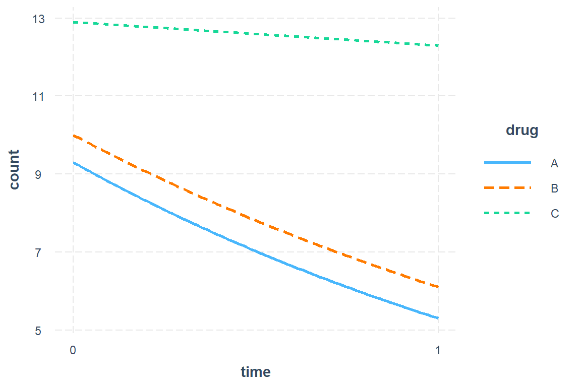

18.4.3.2 Quick

interactions::interact_plot(model = mod_geeglm_exc,
                            pred = time,
                            modx = drug)

18.4.3.3 More Polished

mod_geeglm_exc %>% 
  emmeans::emmeans(~ drug*time,
                   type = "response")

 drug time rate   SE  df asymp.LCL asymp.UCL
 A       0  9.3 1.43 Inf      6.88     12.57
 B       0 10.0 1.57 Inf      7.34     13.62
 C       0 12.9 1.19 Inf     10.77     15.45
 A       1  5.3 1.39 Inf      3.17      8.87
 B       1  6.1 1.85 Inf      3.37     11.04
 C       1 12.3 2.14 Inf      8.74     17.31

Covariance estimate used: vbeta 
Confidence level used: 0.95 
Intervals are back-transformed from the log scale

mod_geeglm_exc %>% 
  emmeans::emmeans(~ drug*time,
                   type = "response") %>% 
  data.frame()

  drug time rate    SE  df asymp.LCL asymp.UCL
1    A    0  9.3 1.429 Inf     6.882    12.567
2    B    0 10.0 1.575 Inf     7.344    13.616
3    C    0 12.9 1.187 Inf    10.771    15.449
4    A    1  5.3 1.393 Inf     3.166     8.872
5    B    1  6.1 1.846 Inf     3.370    11.040
6    C    1 12.3 2.145 Inf     8.739    17.312

mod_geeglm_exc %>% 
  emmeans::emmeans(~ drug*time,
                   type = "response",
                   level = .68) %>% 
  data.frame() %>% 
  dplyr::mutate(time_name = case_when(time == 0 ~ "Pre",
                                      time == 1 ~ "Post") %>% 
                  factor(levels = c("Pre", "Post"))) %>% 
  dplyr::mutate(drug_name = fct_recode(drug,
                                       "Antibiotic A" = "A",
                                       "Antibiotic B" = "B",
                                       "Placebo" = "C")) %>% 
  ggplot(aes(x = time_name,
             y = rate,
             group = drug_name %>% fct_rev,
             color = drug_name %>% fct_rev)) +
  geom_errorbar(aes(ymin = asymp.LCL,
                    ymax = asymp.UCL),
                width = .3,
                position = position_dodge(width = .25)) +
  geom_point(position = position_dodge(width = .25)) +
  geom_line(position = position_dodge(width = .25)) +
  theme_bw() +
  labs(x = NULL,
       y = "Estimated Marginal Mean\nNumber of Leprosy Bacilli at Six Sites of the Body",
       color = NULL) +
  theme(legend.position = c(0, 0),
        legend.justification = c(-0.1, -0.1),
        legend.background = element_rect(color = "black"))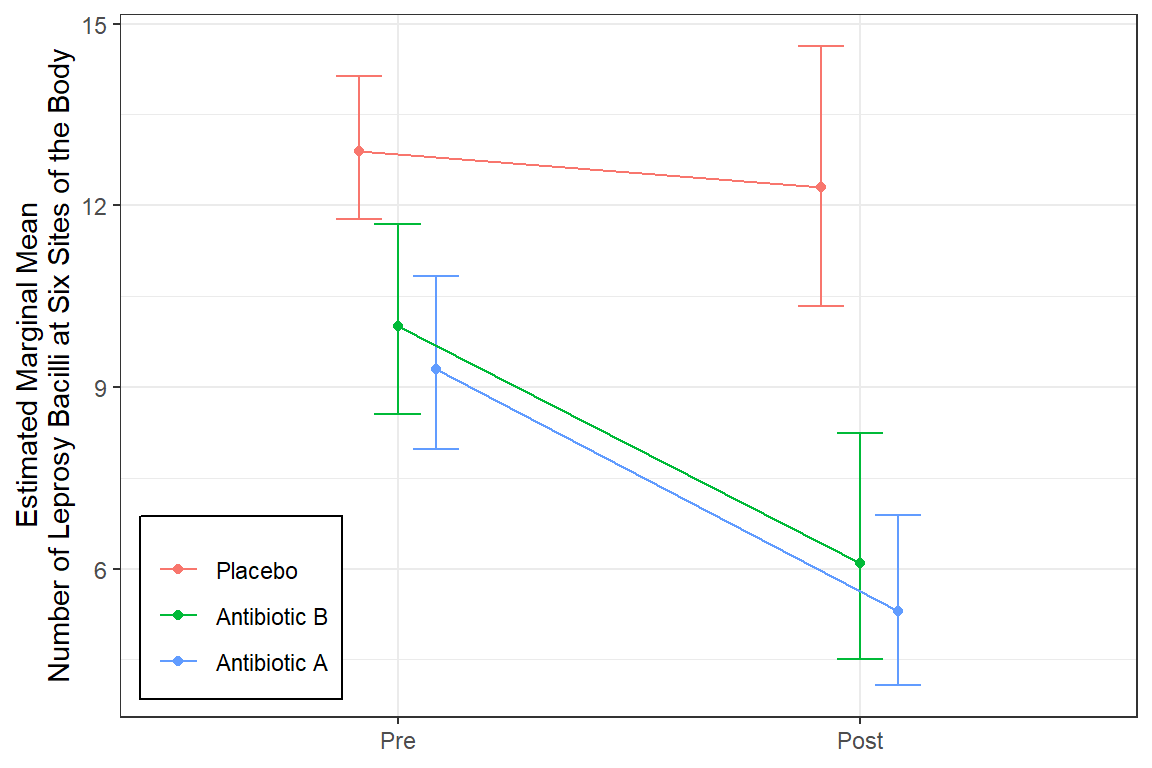

18.5 Follow-up Analysis

18.5.1 Collapse the Predictor

data_remodel <- data_long %>% 
  dplyr::mutate(antibiotic = drug %>% 
                  forcats::fct_collapse(yes = c("A", "B"),
                                        no = c("C")))

18.5.2 Reduce the Model - `gee::gee()`

mod_gee_exc2 <- gee::gee(count ~ antibiotic:time ,
                         data = data_remodel,
                         family = poisson(link = "log"),
                         id = id,
                         corstr = "exchangeable")

       (Intercept) antibioticyes:time  antibioticno:time 
            2.3734            -0.6329             0.1362

summary(mod_gee_exc2)


 GEE:  GENERALIZED LINEAR MODELS FOR DEPENDENT DATA
 gee S-function, version 4.13 modified 98/01/27 (1998) 

Model:
 Link:                      Logarithm 
 Variance to Mean Relation: Poisson 
 Correlation Structure:     Exchangeable 

Call:
gee::gee(formula = count ~ antibiotic:time, id = id, data = data_remodel, 
    family = poisson(link = "log"), corstr = "exchangeable")

Summary of Residuals:
    Min      1Q  Median      3Q     Max 
-9.6185 -4.7333 -0.4843  3.5167 12.3815 


Coefficients:
                   Estimate Naive S.E.  Naive z Robust S.E. Robust z
(Intercept)         2.37335     0.1028 23.07801     0.08014 29.61589
antibioticyes:time -0.52487     0.1024 -5.12426     0.11124 -4.71827
antibioticno:time  -0.01076     0.1142 -0.09421     0.15722 -0.06842

Estimated Scale Parameter:  3.405
Number of Iterations:  5

Working Correlation
       [,1]   [,2]
[1,] 1.0000 0.7803
[2,] 0.7803 1.0000

18.5.3 Compare Parameters

texreg::knitreg(list(extract_gee_exp(mod_gee_exc), 
                     extract_gee_exp(mod_gee_exc2)), 
                custom.model.names = c("Original",
                                       "Refit"),
                single.row = TRUE,
                digits = 3,
                ci.test = 1,
                caption = "Estimates on Count Scale (Exchangeable)")

Estimates on Count Scale (Exchangeable)
	Original	Refit
(Intercept)	9.300 [6.882; 12.567]^*	10.733 [9.173; 12.559]^*
drugB	1.075 [0.699; 1.655]
drugC	1.387 [0.977; 1.970]
time	0.570 [0.404; 0.805]^*
drugB:time	1.070 [0.661; 1.734]
drugC:time	1.673 [1.086; 2.578]^*
antibioticyes:time		0.592 [0.476; 0.736]^*
antibioticno:time		0.989 [0.727; 1.346]
Dispersion	3.474	3.406
^* Null hypothesis value outside the confidence interval.

18.5.4 Interpretation

The grand mean is a count of 10.73 at pre-treatment.
The mean count dropped by about 40% among those on antibiotics, but there was no decrease for those on placebo pills, exp(b) = 0.592, p < .05, 95% CI [0.476, 0.74].

18.5.5 Visualize

18.5.5.1 Refit with `geepack::geeglm()`

mod_geeglm_exc2 <- geepack::geeglm(count ~ antibiotic:time,
                                   data = data_remodel,
                                   family = poisson(link = "log"),
                                   id = id,
                                   corstr = "exchangeable")

18.5.5.2 Quick

interactions::interact_plot(model = mod_geeglm_exc2,
                            pred = time,
                            modx = antibiotic) +
  theme_bw()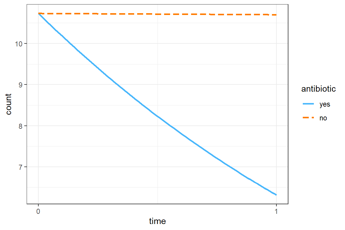

18.5.5.3 More Polished

mod_geeglm_exc2 %>% 
  emmeans::emmeans(~ antibiotic*time,
                   type = "response",
                   level = .68) %>% 
  data.frame() %>% 
  dplyr::mutate(time_name = case_when(time == 0 ~ "Pre",
                                      time == 1 ~ "Post") %>% 
                  factor(levels = c("Pre", "Post"))) %>% 
  ggplot(aes(x = time_name,
             y = rate,
             group = antibiotic,
             color = antibiotic)) +
  geom_errorbar(aes(ymin = asymp.LCL,
                    ymax = asymp.UCL),
                width = .3,
                position = position_dodge(width = .25)) +
  geom_point(position = position_dodge(width = .25)) +
  geom_line(position = position_dodge(width = .25)) +
  theme_bw() +
  labs(x = NULL,
       y = "Estimated Marginal Mean\nNumber of Leprosy Bacilli at Six Sites of the Body",
       color = "Antibiotic A or B") +
  theme(legend.position = c(0, 0),
        legend.justification = c(-0.1, -0.1),
        legend.background = element_rect(color = "black"))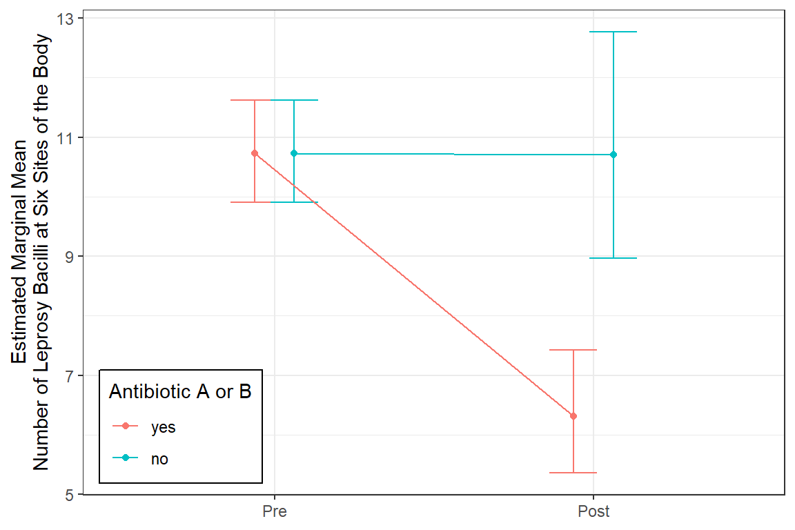

mod_geeglm_exc2 %>% 
  emmeans::emmeans(pairwise ~ time | antibiotic,
                   adjust = "none")

$emmeans
antibiotic = yes:
 time emmean     SE  df asymp.LCL asymp.UCL
    0   2.37 0.0801 Inf      2.22      2.53
    1   1.84 0.1635 Inf      1.52      2.16

antibiotic = no:
 time emmean     SE  df asymp.LCL asymp.UCL
    0   2.37 0.0801 Inf      2.22      2.53
    1   2.37 0.1774 Inf      2.02      2.72

Covariance estimate used: vbeta 
Results are given on the log (not the response) scale. 
Confidence level used: 0.95 

$contrasts
antibiotic = yes:
 contrast      estimate    SE  df z.ratio p.value
 time0 - time1   0.5307 0.113 Inf   4.694  <.0001

antibiotic = no:
 contrast      estimate    SE  df z.ratio p.value
 time0 - time1   0.0029 0.157 Inf   0.018  0.9855

Results are given on the log (not the response) scale.

mod_geeglm_exc2 %>% 
  emmeans::emmeans(pairwise ~ time | antibiotic,
                   type = "response",
                   adjust = "none")

$emmeans
antibiotic = yes:
 time  rate   SE  df asymp.LCL asymp.UCL
    0 10.73 0.86 Inf      9.17      12.6
    1  6.31 1.03 Inf      4.58       8.7

antibiotic = no:
 time  rate   SE  df asymp.LCL asymp.UCL
    0 10.73 0.86 Inf      9.17      12.6
    1 10.70 1.90 Inf      7.56      15.2

Covariance estimate used: vbeta 
Confidence level used: 0.95 
Intervals are back-transformed from the log scale 

$contrasts
antibiotic = yes:
 contrast      ratio    SE  df null z.ratio p.value
 time0 / time1   1.7 0.192 Inf    1   4.694  <.0001

antibiotic = no:
 contrast      ratio    SE  df null z.ratio p.value
 time0 / time1   1.0 0.157 Inf    1   0.018  0.9855

Tests are performed on the log scale

18.6 Conclusion